This may be a kind of silly question, but I would be curious to know about the differences between these probabilistic tracking algorithms. Beyond the fact that they use a different input image (fod vs dwi), what exactly do they do differently, in short? Also, are there situations when one would be used over the other or do they all perform equally well? Thanks!
Directly samples from the FOD interpolated at the current point as a probability distribution: Directions with high FOD amplitudes are more likely to be tracked, but directions with small FOD amplitudes will still occasionally be tracked. Note that this corresponds to directions, not fixels: iFOD1/2 don’t involve fixel segmentation in any way, they use the FOD spherical harmonic coefficients directly.
First-order algorithm: Samples a direction and takes a step in that direction. Consequently will over-shoot in curved pathways.
Directly samples from the FOD interpolated at multiple points.
Second-order algorithm: Each “step” is in fact an arc through space, along which the FOD is sampled at multiple points (-nsamples option). At each spatial point along the arc, the amplitude of the (interpolated) FOD at a tangent to the arc is calculated; these are multiplied to form a probability of traversing along that arc. Reduces overshoot in curved bundles compared to iFOD1.
-cutoff value applies to FOD amplitude.
Tensor_Prob:
For each individual streamline, new DWI data for each voxel are generated based on a wild bootstrap of the tensor model (the tensor model is fit linearly, then the residuals of the model are randomly flipped and added back to the original signal). At each streamline vertex, interpolate the (bootstrapped) DWI data at that point, fit the tensor model, and step along the direction of the principal eigenvector.
Either first- or fourth-order: Will have curvature overshoot by default, but can be combined with fourth-order Runge-Kutta integration via -rk4 option to greatly minimise this effect.
-cutoff value applies to FA (of the tensor model as estimated at each streamline vertex from interpolated bootstrapped DWI data; not a pre-calculated FA mask).
Would only advocate the use of Tensor_Prob in the specific case of demonstrating how bad it is (this is the only reason it’s implemented). iFOD2 is conceptually superior to iFOD1; some people have their criticisms, but trying to fully explain the nuances of their differences only to attract more questions about which to use would be counter-productive. So unless you are actually fully aware yourself of all of these differences, or are wanting to explicitly devise an experiment comparing them, best to just stick with the default iFOD2.
I guess the choice of algorithm also depends on the available data, right? On HARDI data, the iFOD1/2 will work fine, but on ‘DTI’ data (e.g. 30 directions b=1000), a Tensor algorithm may work better. This is just my assumption, correct me if I’m wrong.
Well, this depends entirely on how well the FODs are estimated – but in my experience, we can get reasonable looking results even with these types of data, providing the SNR is sufficient. Indeed, I’ve got non-terrible looking outputs from 12 direction b=1000 data… I’m not suggesting that these types of data are sufficient, but they can be processed with CSD / iFOD1/2 with decent results (considering how far from ideal these data are), although it will probably require some tweaks to the parameters (mostly setting -lmax 8 in the dwi2fod call, probably others too).
I’m not sure I’d ever say that a tensor algorithm ‘works better’ in the context of tractography… It might give you much cleaner-looking tractograms, but 'll always be affected by crossing fibres, whichever way you look at it. CSD at least has the potential to give you relatively unbiased fibre estimates even with substandard data. The main issue with CSD in these ‘DTI’ data sets is mostly the relatively poor contrast to noise, which basically means noisier tractography (potentially much noisier, to be fair…).
Thank you for such thorough replies, they have indeed cleared things out. However, I just wanted to show you the results on my data, and maybe determine whether the results that I am getting with iFOD1/2 are “decent” results, especially given that they seem to be completely different compared to the Tensor algorithm.
Firstly, the data is aquired with 32 directions and a b value of 1000, so not of great quality.
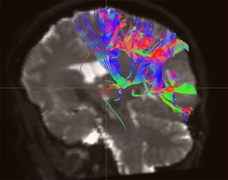
Using the iFOD2 algorithm I get 82630 streamlines which look like this:
OK, this is a slightly unusual way of assessing tractography – I’ll try to (briefly) explain why:
Raw streamline counts are essentially meaningless (as eloquently explained by Derek Jones). It is certainly not an easily interpreted measure of ‘quality’.
If we were to make sense of it, we could only do so in the context of the specific commands issued, the ROIs used, and all of the other relevant parameters. In particular, you must have used non-default values for the -select or -seeds option – and I assume you used the -seeds option…? If you want an opinion on your results, please provide the full command-line used to perform the tracking in each case.
it’s very difficult to compare deterministic tensor tracking to probabilistic non-tensor tracking – they’re very different approaches, which makes a direct comparison problematic. The interpretation of results is quite different. A probabilistic algorithm will always, by design, produce more widespread streamlines, what matters is which pathways are ‘densest’ (and even then, it’s not that clear-cut). An approach designed to resolve crossing fibres will also allow the algorithm to produce more potential pathways: there’s more directions to choose from at each step.
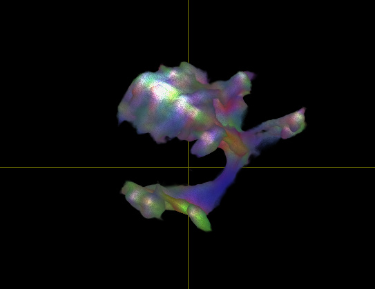
For your final render to work, you’ll need to adjust the ‘transparency’ & ‘alpha’ settings in the View tool. In your screenshot, the low intensity (low ‘probability’) regions obscure the dense parts of the pathway. Try increasing the lower value for the transparency to make those low intensity regions transparent.
Thank you for your answer, I’ll try to make things a little bit clearer:
In both pictures I used the same inclusion ROIs (language-relevant TMS stimulation points), and basically the command was identical in both cases, with the algorithm being the only thing that is changed (and the input image):
(The cutoff FA and minlength are at those values quite randomly - later on I would like to compare between various values of these and how they would influence the visualization of the tracts.)
Should I have used the “-seeds” option? How would that improve the results and how would I choose an adequate number of seeds?
I did not use deterministic tensor tracking, but the probabilistic version (Tensor_Prob), mainly because the iFOD2 tracks so much that it is hard to see the “order” underneath, or else I would have of course not even tried to use an alternative. My only purpose would be to use a probabilistic algorithm and not a deterministic one, and if I could somehow make it work with iFOD2 that would be the best case scenario…
With the updated transparency settings, I still get a somewhat blurry image, is this simply how it is supposed to look?.. As I am dealing with tract identification, it becomes very hard when the image is not as “sharp” as the result from tensor_prob, for example.
Again, many thanks for taking the time to answer…For a beginner Mrtrix is daunting to say the least, but with such a helpful community it feels easier to push on.
Ok, that’s strange. By default, tckgen will try to generate 5,000 streamlines, and keep seeding until that number have been selected (equivalent to -select 5000). I find it very strange that you’d get more than that number with the commands you’ve used. I note there’s also no seed specified…? Are you sure these are correct? What does tckinfo show for the two tracks files?
No, whether you use the -select or -seeds option depends entirely on what you’re trying to achieve in your research. I don’t think it would make any difference to the ‘quality’ of the results – but it would explain the discrepancy in the numbers, which is the only reason I raised it.
So you did. Sorry, my mistake…
I guess this is the primary issue here. Display of probabilistic results can be difficult if you’re used to much ‘cleaner’ results. A big contributor here is the very large number of streamlines you’re trying to display. With that many, it’s easy for the low probability, noisy outliers to obscure the deeper, denser, and presumably more relevant bundles – you can’t see the wood for the trees… For a single seed like this, I would have thought that 5,000 would have been more than enough.
Also, this is where the ‘crop to slab’ visualisation works best: it allows you to look at the streamlines within the anatomical plane of interest, and the superficial noisy streamlines won’t interfere so much. It also makes it much easier to appreciate exactly where the streamlines pass relative to the anatomy. A bit of transparency can also help here.
Well, I’m sure we can improve on its appearance somewhat, but at least you can now see where the main bundle is going (is that seeding from Broca’s, pulling out the arcuate?). Is that what you were expecting?
Also, it’s supposed to be blurry, at least to some extent: a probabilistic algorithm should give you you a distribution of likely pathways, especially when relatively unconstrained (e.g. single seed experiment). Any noise or other source of uncertainty will (rightly) make the results blurrier.
In terms of display, you could probably do better by loading a coregistered T1 as the main image, and the colour TDI as an overlay, then add a few clip planes to reveal the tractography results in their anatomical context.
But to be able to help get the best out of your data, we’d need to see all the commands you’ve used, right from the raw data. Did you use denoising? Gibbs ringing removal? Eddy-current and motion correction? Correction for EPI distortions? Regular or multi-shell CSD? With what parameters? ACT during tracking? There’s lots that can be done to improve and refine the results…