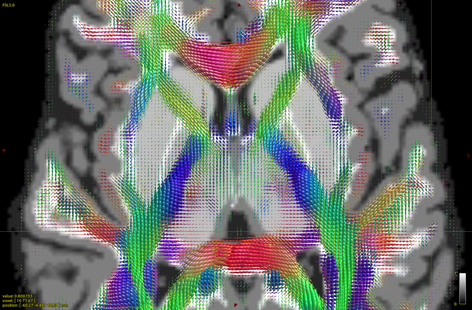
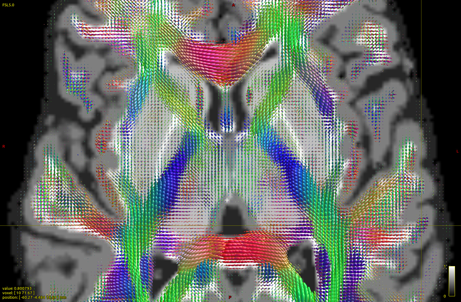
I ran a subject (2x2x2 mm resolution, b0 vols + 60-dir b=700 AP+ 60-dir b=700 PA+ 60-dir b=3000 AP+60-dir b=3000 PA, generating after the dwiproproc recombination a b0+60 vol b=700+60 vol b=3000 multishell mif image) with either the dhollander or the msmt_5tt algorithm:
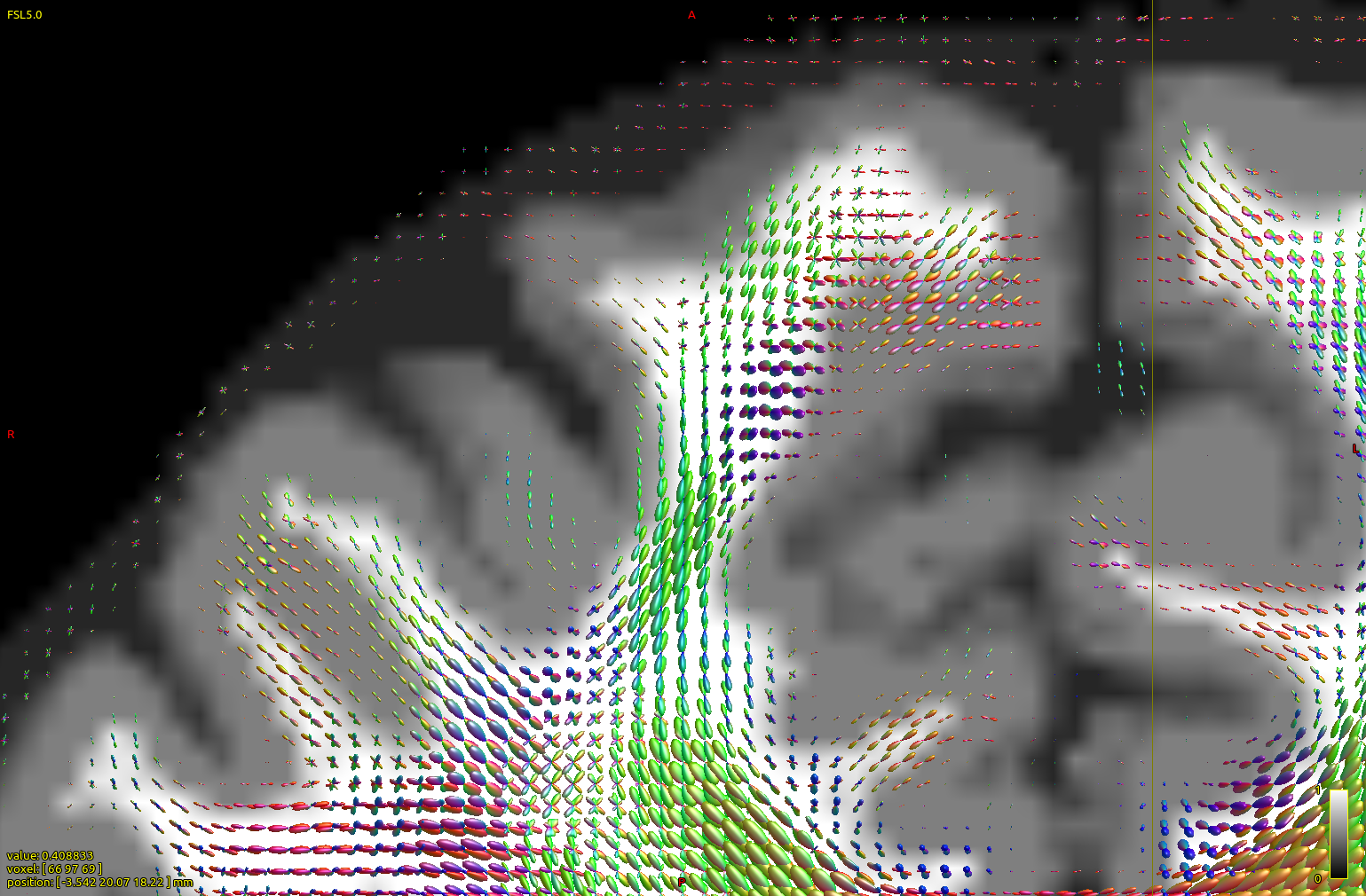
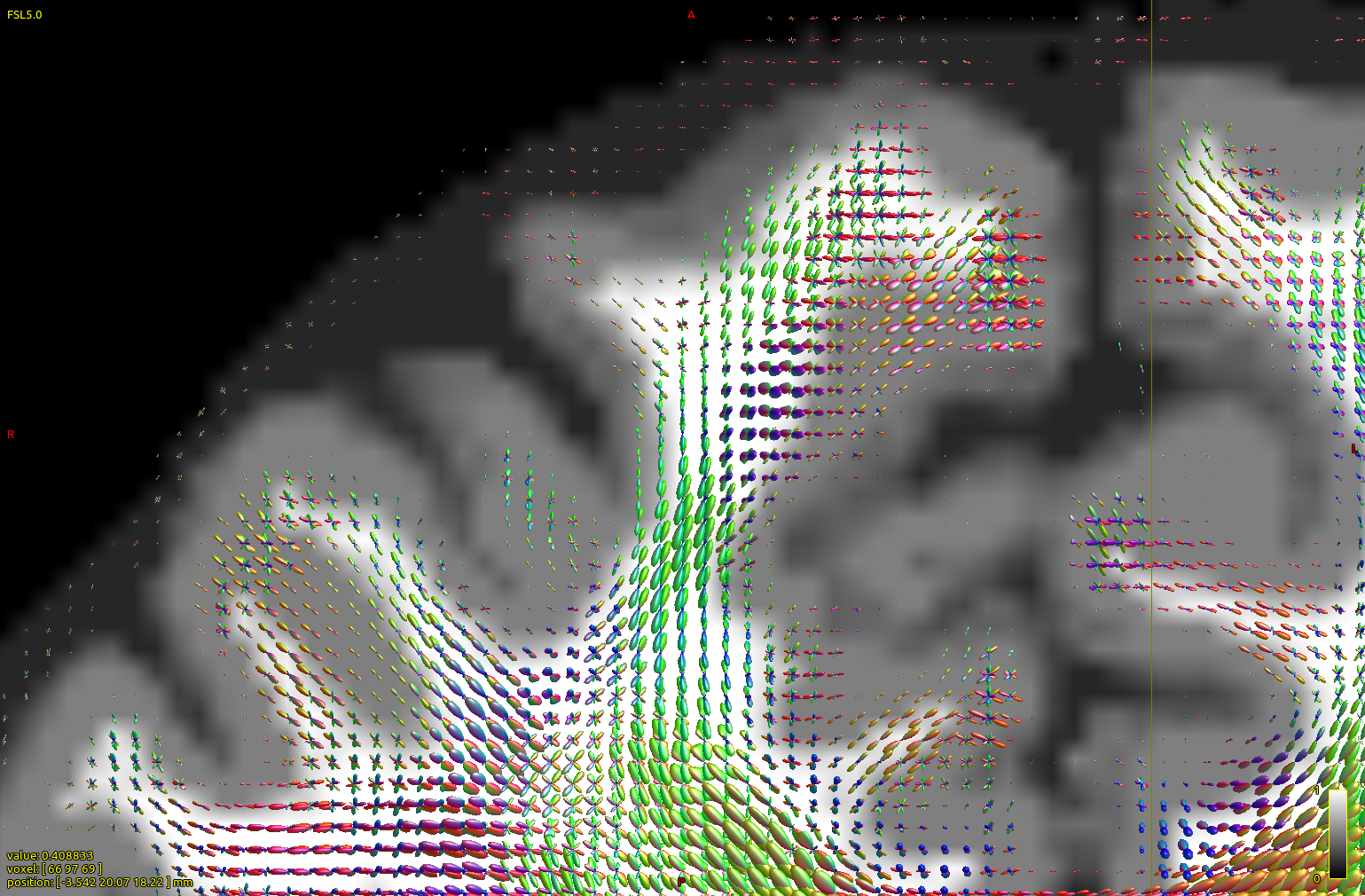
The top image is dhollander output, and the bottom msmt. It is apparent that CC/midline structures such as splenium are fatter in dhol than in msmt and overall dhol looks cleaner, however msmt ODFs seem to extend/branch out more laterally/peripherally. In other words, dhol appearance is more ‘centripetal’ vs msmt ‘centrifugal’. Is this the expected behavior?
Three more questions regarding this:
How is dhollander vs tournier on single shell data, any takes?
If one omits the -lmax flag with dwi2response, either ‘tournier’, ‘dhollander’, or ‘msmt_5tt’, is the default set based on the data (no of volumes, on teh set herein lmax would be 8) therefore one can omit it, or the default lmax is set on a fixed, lower value?
Since one explanation offered for the good dhollander performance vs msmt was the need for the latter for a good T1 registration, are there preferences among mrtrix experts for a verified, well-performing dwi-T1 registration method that we could implement (without guarantees or strings), or is it the wild west? We tried FLIRT/BBRegister and did not see big differences by eye-balling (both methods gererate areas with visible, if small, mismatches), but wanted to know you opinion for more ‘advanced’ (nonlinear) methods (eg. one recently published, regseg) ?
Thank you,
I’ve split off your original reply as a new topic, as it was a bit hidden in an existing topic (that was about another topic ). I hope you don’t mind.
I’ll get back to your questions tomorrow; I’ve got some good answers, but it may take some time to write them up decently… I’ve also got a figure or two to help illustrate some things for you.
In the mean time, a few quick remarks on the commands you’ve posted; as I’m spotting an error in there and I’ve got another piece of advise. It may be best to test (again) using these points, so as to make sure we’re still talking about the same findings:
The -lmax 8,0,0 in dwi2response (both dhollander and msmt_5tt) is wrong: the -lmax option for dwi2response specifies lmax’es for each b-value rather than for each tissue type. For these algorithms, the lmax’es that you specify only apply to the WM response, as the GM and CSF ones are inherently always isotropic (lmax=0) for all b-values. So in your case, this should have been something like -lmax 0,8,8 instead, reflecting the WM lmax for b=0, b=700 and b=3000. However, it’s even better to not supply the lmax option at all! The lmax is now set automatically to 10 for you for all non-b=0 shells of the WM response. Don’t worry about your 60 directions not being enough for that or something: the response is estimated from at least hundreds of voxels, so lmax=10 (and in principle even way beyond) is easily supported for the response functions. So long story short: ditch the lmax option to dwi2response.
I spotted a suspicious -mask mask_dilated.mif option to dwi2response there. The suspicious thing (for me) being the “dilated” there. This may make sense to dwi2fod, so you’re covering a safe extra margin when computing FODs, but for dwi2response this isn’t needed. In fact, this may even be detrimental there: as no useful response functions will ever be obtained from that margin beyond the brain and outer CSF. In extra-fact, dwi2response dhollander even on purpose erodes the brain mask: the definition/intuition of a “safety margin” for the purpose of response functions works quite the other way around: you’ve got loads of voxels in a whole brain mask, so you can be extra-picky about choosing only the best ones. It makes sense to avoid dangerous areas (like the very outer few voxels of a potentially not-entirely-accurate mask) at any cost. Your data looks like relatively normal developed brains, in which case dwi2response will happily compute a decent (enough) brain mask itself, and erode it for you. So long story short for this one: ditch the -mask option to dwi2response as well.
Your dwi2fod call is fine (and correct), but you can safely ditch the -lmax option here too. It’ll manage the lmax’es safely on its own for you.
So I would recommend re-running both dwi2response calls (and then dwi2fod of course as well) without the -mask and -lmax options, and let them do their thing that way.
Maybe a small additional request, so I can help you better (tomorrow when I work on a reply for you): could you zoom into a region (somewhere, anywhere around the cortex). The current screen shots are very hard to look at for those regions, as the resolution (of the screen shot) is quite low. It’s impossible to see what those FODs look like around these areas.
Finally, definitely also provide a copy-paste of the text (numbers) in each response function file (they’re just text files), e.g. as was done in this post. They typically explain much more about your response functions than the FODs (indirectly) do. The interactions in multi-tissue CSD can get quite complicated between the 3 tissue types at times, depending on certain properties of the actual response functions.
Ok, that was already quite some text. I hope my actual reply tomorrow won’t be much longer…
Here are two figures/insets of the left frontal cortex and wm, along with interhemispheric fissure (right margin) and part of ccal (right lower corner). Top figure is dhollander, bottom msmt (detail 3, scale 3, no interpolation, to accentuate differences) over the act_vis.mif structural.
Again, dhollander FODs seem to be better confined to structural wm (with exceptions, such as some portions rich in CSF), while enriched in CCallosum, in contrast, msmt ones are more ‘diffuse’, often with larger lobes at the gmwm junction or in the gm.
Please add these questions to my previous ones:
1/retake: If the default msmt_5tt and dhollander lmax for wm is 10, which is the default for tournier?
2. If we are not to worry for a default lmax of 10 when no or vols/grads would indicate an lmax of 8 for the RF, should this lack of worry extend to the case when the no of images is *much" lower (~30)? This is to cover most bases in case of a pipeline that may be used on image sets with widely different no of gradient directions.
3. when we should expect the dhollander paper out?
4. re dwi/structural registration: in addition to the larger discussion involving many aspects of this kind of registration, is there a tool other than FLIRT/bbregister that has successfully been used in your hands AFTER topup/eddy application (whether or not strictly for b=0/T1 transform)?
Thank you for taking the time to answer all these,
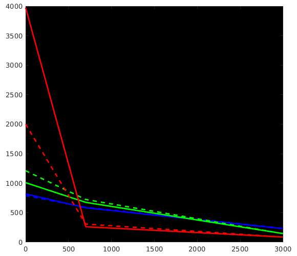
Great stuff, thanks for posting all that! It beautifully reproduces my findings up to now on a lot of datasets, as well as data from a few of other people around here who’ve also wondered about the differences. Let us take a look at how we can perfectly explain everything we see in your results. I did a quick plot of your reported response functions’ b-value dependent behaviour, which makes things a bit more visual (I always recommend taking a look at things like this):
WM-GM-CSF = blue-green-red (as in my abstracts, and also in Ben’s original MSMT-CSD paper), dhollander is full lines, msmt_5tt is dashed lines; horizontal axis is b-value (just 3 discrete points of course; your b-values); vertical axis is amplitude of each response (your numbers, but in general these are arbitrary units).
Ok, so, observations:
WM responses are as good as the same
CSF response function of msmt_5tt has a drastically lower b=0 intensity (compared to dhollander) and minor increase in b=700 intensity
GM response function of msmt_5tt has a significantly larger b=0 intensity (compared to dhollander) and minor increase in b=700 intensity.
What can have impacted msmt_5tt to explain the different CSF and GM responses?
CSF:
Mis-registration of T1 vs DWI data: since CSF has the largest b=0 of all tissues by a wide margin, any (even subtle) mis-registrations will cause selection of “CSF” voxels that are non-CSF tissues, resulting in what can only become a severe drop in b=0 versus what it should have been. msmt_5tt has one additional form of protection, which is an additional FA threshold for GM and CSF (to stay below). This protects it a little bit against these problems where CSF interfaces with WM (high FA) specifically. However, it doesn’t protect against this issue at CSF-GM interfaces. And even at CSF-WM interfaces, it’s very limited in doing so, since “WM” FA drops very easily to quite low levels when even partial voluming only a bit with CSF. So we may still see (and get) voxels there with a low enough FA to make the cut, yet still significantly partial volumed by WM.
Mis-segmentation of tissues that aren’t 100% CSF as still very much close to “100% CSF”. Number one culprit to significantly cause this even in perfectly healthy brains: the choroid plexus structures in the ventricles. While these are sometimes barely decently visible in a T1 image, they are very real structures sitting there and changing the b=0 more than enough to be taken seriously. I note in your dataset, since you’ve also shown the 5tt image in the background (I presume) that in fact some of those got segmented as GM (which is also not what they are, see further on for GM response issues), which at least kept them partially away from the CSF selected voxels (one would hope).
GM:
Mis-registration of T1 vs DWI data: you effectively run the opposite risk compared to the CSF scenario here. You could first assume that this may “average” a bit out in a way: GM is mostly the cortex, which is mostly wedged in between WM and CSF (outside the brain) areas, so some random mis-registration may naturally land you with some GM-segmentation still overlapping (in DWI space) with actual GM, but some also with WM and some with CSF. Let’s naively assume 33% for each tissue type ending up in the “GM” segmentation or something like that… you could then naively assume that this saves the day a bit, since the b=0 of GM also sits in between that of WM and CSF. However, 2 important biases come to ruin the day here: first, the CSF has a much much higher b=0 whereas WM only has a moderately smaller b=0 intensity, so an “average kind of” mis-registration already biases towards the higher b=0. Second, there’s that FA threshold for selecting CSF at the end too, which prevents those accidental inclusions of WM voxels. So the bias will almost uniquely be towards the b=0 of CSF, which is indeed drastically higher than it should be (for GM).
Mis-segmentation of tissues that aren’t 100% GM, or not even GM at all: the cortex is not that wide, so the not quite 100% thing happens very easily. However, the “not even GM at all” is the biggest risk here: about any pathology of WM that lowers “fibre density”-like aspects, or even more so myelination, will result in a lower (than WM) T1w intensity. Think for instance WM hyperintensities in ageing or multiple sclerosis. We’ve got heaps of those over here (in our institute): 5ttgen classifies a lot of that stuff as (almost pure even) GM. However, in practice, it’s often a mix of tissue changes that tend towards a higher b=0 (well, it’s T2 hyperintensities anyway, right) then what you’d even see in healthy GM. Furthermore in your case: there’s the choroid plexus again. Shouldn’t be GM, and at your DWI resolution of 2mm isotropic, it’s going to have lots of partial voluming from CSF. However, an overwhelming amount of your GM voxels will still come from the actual cortex, so the choroid plexus isn’t going to be responsible for much problems in your case.
In practice, for your example, I reckon both “mis-registration” scenarios have played out, and to a (much) lesser extent the "mis-segmentation ones. I note for instance also a band of “GM” segmented at the interface of the thalamus and the CSF. I can see how that could’ve come from the T1, although it’s wider then what I’d expect: maybe you had an anisotropic T1w resolution? Or the T1 was blurry otherwise? I’d expect to see a band like that, just not that wide. Again, the CSF’s T2 will overwhelm there, and bias your GM response towards CSF properties.
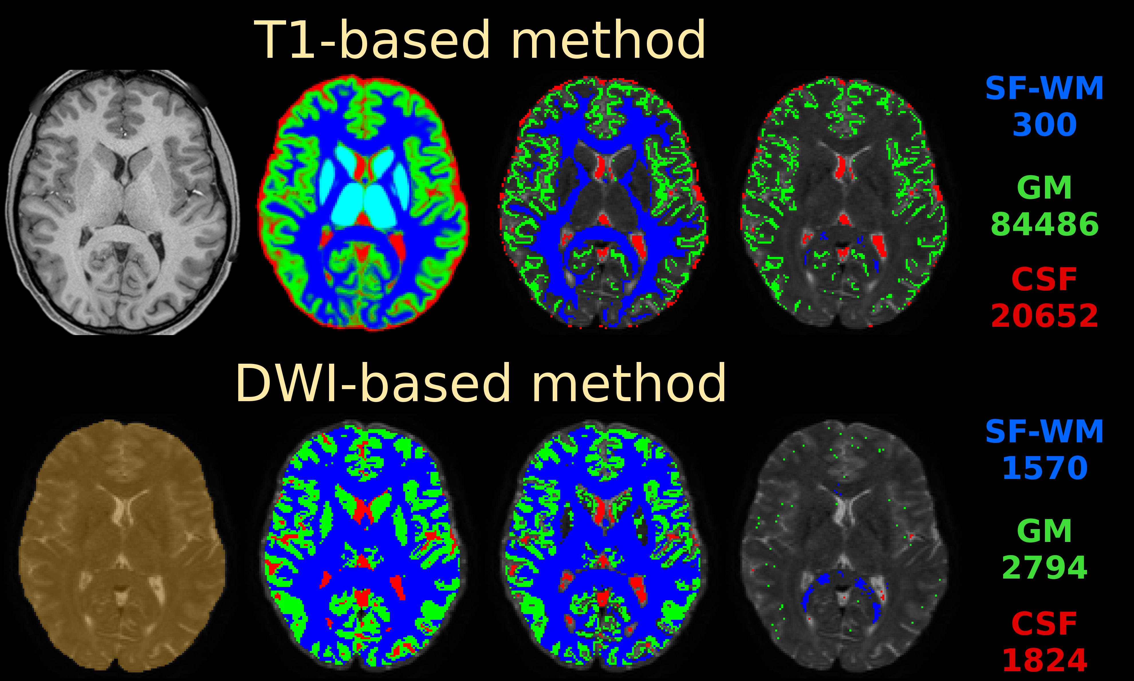
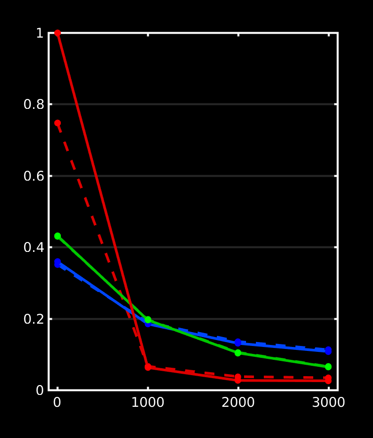
If you do nail registration as good as realistically possible (combined with the best image quality imaginable), you may be able to reduce msmt_5tt’s GM problems. Note they weren’t apparent in the data I presented in that abstract. I’ve also pushed this to high quality data, by using the preprocessed HCP data. I reason that’s quite up there in terms of data and preprocessing quality. See here the results of such a dataset:
Top row is msmt_5tt going through some steps (final column is the final voxel selection in diffusion space), bottom row is dhollander going through the same “main” steps as presented in the abstract. These are the responses that came out here:
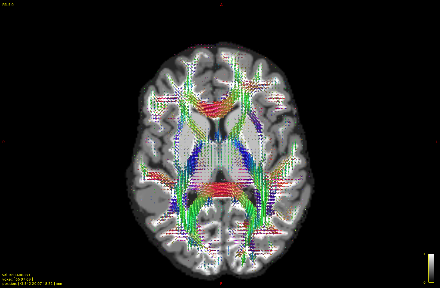
Note the WM and GM are basically the same between both algorithms (even though the selected numbers of voxels for those 2 tissues were very different; this is good news in general, it does show that in good conditions the 2 very independent strategies go to a consensus… reassuring!). Note that the CSF still suffers from the problem described in the abstract (and reproduced on the forums here already a couple of times by people, and by your data now as well). If we assume very good registration quality in the HCP case, then segmentation issues it is: note the final CSF voxel selection for msmt_5tt’s CSF is still quite generous, and indeed includes the choroid plexus and a lot of risky voxels at the edge of the mask. The dhollander algorithm is much more picky, and goes directly with the diffusion data’s properties (actually looking for a sharp decay as is expected for free diffusion). Look how it nicely avoids the choroid plexus and anything that even barely risks being partial volumed. But the dataset is so large, we can easily afford being this picky: we’ve still got 1824 CSF voxels (and lots of images per b-value) to work with. That should be more than enough to estimate just one average number for each b-value. After all, this is not about a segmentation to begin with: it’s about a very picky selection. (to see the full selection of voxels from dhollander for this HCP dataset in 3D, see the screen shot posted here)
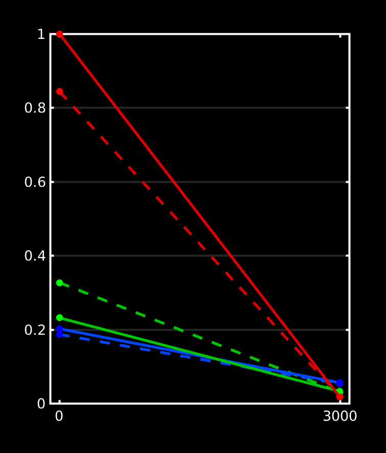
Here’s the responses I got over here on a dataset (with a more realistic spatial resolution), yet with some lesions:
I can’t disclose much of the other results on these datasets at this point, but essentially lesions got selected as GM by 5ttgen, and hence the GM response function selection by msmt_5tt came mostly from those areas. Note the now very expected CSF problem also pops up (of course, as always). There we’re also slight mis-registrations in place here, due to partially uncorrected EPI distortions (motion / eddy currents were corrected though). Again, everything with the expected effects on the response functions.
Next, consequences for your FOD estimation when using your responses. I’ll talk in terms of biases caused by the biased GM and CSF responses that resulted from msmt_5tt. To understand this, it’s useful to consider tissue interfaces, because that’s where the contrast between 2 tissues will go wonky if either (or both) responses aren’t appropriate for what they’re supposed to represent. Here’s all the interfaces:
WM-CSF: troubles here caused by the underestimated CSF b=0, or in general underestimated CSF diffusivity. This scenario is mostly described in the original abstract. Essentially: more “CSF” is needed to represent the b=0 signal using the CSF response that has too little b=0. It’s actually more about b=0 versus the other b-values, and hence about the diffusivity, but the argument has the same format. The opposite holds for the WM response contribution here (even though the culprit is the CSF response, but it’s all about relative balance between both). Result: underestimation of your WM FOD, and it sometimes disappearing entirely for some levels of CSF partial voluming. Your responses and the resulting effect at the WM-CSF boundary is actually one of the most severe I’ve every seen. Don’t underestimate the impact for subsequent applications: e.g. the midbody of the corpus callosum (that is already quite a thin structure relative to DWI resolutions) is impacted severely, on both sides, so it grows significantly “thinner”. This impact quantification of FD, FC and FDC for this structure, and may cause strong biases in any connectome (as a significant number of the left-right connections of the brain go through this crucial bridge). Furthermore, in pathology (e.g. lesions), this may overestimate the free water content, and sometimes severely underestimate the amount of healthy intra-axonal space left. Pretty risky if e.g. surgery is informed by that.
WM-GM: troubles due to overestimated GM b=0. The (or a) simple(st) way to reason about this is to think of the GM response having become a bit more CSF-like. So the behaviour at the cortex becomes a little bit more like the scenario where we would have no GM response (i.e. 2-tissue CSD with WM and CSF). So essentially, some isotropic GM signal that would otherwise be captured by the GM response, is now not. And too much signal ends up in the WM compartment, which is your WM FOD. You can see this, as you’ve described, by larger FODs there… but note that in most cases in your more detailed zoomed screen shots, you can observe that these are messy FODs, or messy additions to FODs that were cleaner in the dhollander case. This is the “fingerprint” of isotropic signal being deconvolved by an anisotropic WM response, while using an SH basis that is cut off at a certain lmax. If you deconvolve perfectly isotropic signal that has just a tiny, tiny bit of noise on it with an anisotropic WM response, you don’t get a nice isotropic FOD, but a sphere full of random peaks. The noise is sharpened, and the SH result goes up and down like crazy. Not a useful addition to your WM FOD in those regions, that is… Again in case of pathology (again e.g. lesions), this may underestimate e.g. gliosis, and have some of its effects messing with your WM FODs. You also end up overestimating AFD then in these regions, and hence underestimate some of the damage in case of a genuine lesion.
GM-CSF: we can’t see this going with just your WM FOD; the GM and CSF outcome maps may show some effects here (in addition to those at the other interfaces described above). But both GM and CSF responses are biased towards each other… so you may see a (false) over-contrast of the GM-CSF spectrum. It’s as if you set the windowing on an image too tight in a way. The balance may also be disturbed dependent on which bias (of both responses) “wins out”. In pathology… well, this becomes a mess.
Finally, note that in general both of these GM and CSF response function biases strictly reduce the range of signals you can fit (even independent of meaning and interpretation). See for instance Figure 5 in this recent abstract: the triangle in the right hand side schematic will strictly shrink due to either of those biases. This schematic has actually already helped me a lot to translate formal observations about the response functions as well as 3-tissue CSD into visual interpretations, and more intuitive explanations. Using that schematic, you can perfectly obtain the above explanations at tissue boundaries under the presence of a response function bias as well. It’s a mighty handy tool (if I say so myself ) for white board discussion marathons (and my boss/supervisor has a big one in his office, so fun times guaranteed ). Also, both the inner workings of my SS3T-CSD as well as even the strategy of the dhollander algorithm can be made very visual on that actual schematic.
Alright, if I continue like this, I may end up with the actual paper almost written. I’ll briefly get to your questions, so I don’t overlook anything you were looking for:
This should now be clear from the above. Especially important for e.g. corpus callosum and fornix.
So from the above: be very careful about this, as a lot of this seems to be “false positive signal” that shouldn’t have ended up in the WM FOD, but rather in the GM compartment. Some of in in your zoomed screen shot is particularly messy, and also quite big compared to the actual nearby deeper WM. Not surprising: if this signal now ends up in the WM FOD, but has to be modelled by the WM response’s lower b=0 value, it’s going to be over-represented even more.
Even though both GM and CSF response biases of msmt_5tt work together in your case to give you this appearance (of dhollander versus the biased msmt_5tt), this isn’t a representation of both of them being more suited towards a certain region. Bigger FODs aren’t always better, as we’ve seen from our WM-GM boundary reasoning.
This is somewhat unrelated to all of the above. First things first: at the moment dhollanderusestournier internally for the final single-fibre WM selection, but dhollander already narrows things down for tournier to a safer selection of WM (both single-fibre as well as crossings and other geometries still). dhollander also determines a more relative number of voxels (compared to WM size and resolution) that scales better in case of pathologies or varying spatial resolutions, and then asks tournier for that. tournier out of the box (default) always goes for 300 voxels, independent of anything. You can set this number yourself of course as well if you run tournier. But in general, the core of the strategy to identify the single-fibre voxels is the same. In practice, for a single-shell response they also tend to give a very similar result. For multi-shell purposes though, tournier ignores lower (and b=0) b-values. dhollander has a sneaky outlier-rejection going on to avoid pesky CSF-partial volumed voxels and other unexpected T2 hyperintensities. This does help it to get slightly better multi-shell (or even b=0 and single-shell) response for WM. But this doesn’t matter for single-shell single-tissue CSD: for that one, only the shape of the response is the crucial thing. No drastic differences here. I’d advise to simply run tournier directly if you need a single-shell single-tissue CSD response. No need to overcomplicate things for that scenario. In the future, there is a chance that I change what dhollander does at this stage. It’ll always be inspired by the general strategy of tournier though, but there’s a few other things of concern going on, and an opportunity to slightly improve the multi-shell (or b=0 + single-shell) WM response; but I need to figure out if I can get it ultimately robust. (robustness is a property of the dhollander algorithm that I’d personally never want to sacrifice)
At the moment, the default for all algorithms will inherently end up being lmax=10. That is, for all WM responses (GM and CSF have lmax=0) and only for the non-b=0 shells of that WM response (again, b=0 has lmax=0). See some experiments and discussions and equally lengthy stand-alone posts on this: here, here and here are some relevant bits, but happily read that entire page of discussion (they’re all bits on the same page). If you’ve got any further questions on that front, don’t hesitate to ask for clarification. But the gist is: even with crappy 12 direction data (imagine that), and even with only 100 voxels for the single-fibre WM response (that’s a lot less than what you’d realistically always get), you’ve still got 1200 measurements, to estimate just 6 parameters (that’s the lmax=10 response model, i.e. lmax=10 for a zonal spherical harmonic basis). On top of that, we’ve got non-negativity constraints and monotonicity constrains for the WM response (if those 1200 measurements weren’t already enough to estimate just 6 parameters). And lmax=10 is certainly more than flexible enough to represent responses up to b=5000 in vivo. So it’s flexible enough, and mighty safe given the massive amounts of data we always have for this task.
As mentioned above, even a perfect registration doesn’t overcome all issues. But for it to at least be as perfect as possible, you’d need it to be sub-voxel accurate (relative to the DWI spatial resolution). And of course, up to that same level of accuracy, be able to overcome the many distortions that plague EPI data. And even then still, msmt_5tt will trip up over mis-segmentations… all while the actual information about the actual responses you’re after is actually right there in the DWI data, rather than in a T1. Note that the msmt_5tt algorithm was never meant to be the ultimate way of doing things; but at the time there was certainly need for at least some automated need to do this. It would otherwise have sounded very arbitrary in the paper(s) that we picked our responses “manually”… it also wouldn’t have been very convenient in practice to do this on cohorts of many tens or hundreds of subjects. msmt_5tt certainly did what it needed to do at the time. However, your question (about registration) remains important: for tasks like ACT, you still want that registration to be as good as it can get of course. It may be worthwhile asking that one specifically again in its own topic (with a well chosen title) to get some input from other peoples’ experience. I’ve seen a few different things here an there on the forum before too.
I should have read all question before I started typing above. So, as mentioned in the other answer: it’s also 10.
Yep, no worries, as mentioned in that other answer above. You’d even get away with 12 directions (or less!). However, the question you’ve got to ask for such a pipeline is what lmax for the CSD step is till appropriate, or even if the CSD step itself is still reasonable. But the response function estimation is (un)surprisingly safe. Also be careful with the results of such a pipeline on data with such differing qualities, as in: don’t compare such results with each other (i.e. based on different qualities relative to each other).
Looks like I almost wrote it in this post now. But other than that: it is my first and foremost priority at the moment, even before any SS3T-CSD shenanigans. Other projects (well, collaborations) do run in parallel, but those are now bootstrapped sufficiently (I hope). Time to focus on this one; lock myself up without internet and with a typewriter.
Again, very useful as a topic of its own; I expect different experiences in the wider MRtrix3 community. I’m always happy to learn what people do for these steps as well!
Sorry to open again this old topic. I have a couple of small question regarding the mask used for dwi2response dhollander and the default values of-cutoff
I work with neonatal data, and I create the masks using the dHCP pipeline. This masks are quite good, removing almost all the external CSF. I noticed that the mask is always eroded in the response function algorithm, I thought that if the mask was entered manual this was not the case, and I was eroding the mask before passing it (-npass 2), as a result the eroded_mask has been eroded 5 times (2 before and 3 during the dwi2response function). The response functions are almost identical, but just to double check, do you think this will have a major impact in the tractography?
And another small question. the default value of -cutoff for tckgen is 0.06, this is for multi tissue responses function, if I plan to use only two responses (WM and CSF), should I change this parameter, even if I always run mtnormalise? Thanks in advance.
No worries. 2 very different topics though (just to be clear for future readers of these posts ). Here we go:
That’s a good start indeed; definitely good to use a reliable method, check the masks, and manually (or otherwise) correct when needed. Some methods, including dwi2mask (when it works well at least), do aim to actually have the external CSF included in the mask. It doesn’t really matter if all you analyse is the brain parenchyma, but it’s worthwhile to note, since some methods are designed or slightly tweaked to “expect” such masks. However, in this case, it doesn’t really matter all that much (see further below), so no worries.
That’s correct, and entirely intended. I know other algorithms might not do this, but in the dhollander algorithm, this is on purpose / by design. The idea is indeed that you might get you mask from any brain mask estimation algorithm yourself, which still provides a whole brain mask that might indeed go all the way to a certain outer edge, e.g. the outer cortical surface or even further e.g. including the external CSF. Since the algorithm doesn’t need the whole brain, but only safe/pure voxels after all, it can (and should) just play “as safe as possible” by default, and thus erode to stay away from potentially misleading voxels at all costs. If your mask estimation procedure is already very “conservative” / safe, or as in your case, you’ve actively eroded it yourself with that intention, you can switch off the erosion by the dhollander algorithm by using its own -erode option and actively setting it to 0, i.e. -erode 0. However, …
As you observe indeed, it has almost no impact, and that’s a good thing: those few extra outer “layers” of voxels that get eroded (or not) shouldn’t crucially matter in most cases: there are still plenty of good examples of the “purest” voxels deeper within the mask in any case. Since almost all steps of the algorithm are non-parametric, it can deal with changes in balances between numbers of voxels in respective tissue types, e.g. due to extra erosions, but also severe atrophy, lesions, tumours, surgical resections, etc… So in your case, by effectively eroding 5 times in the end, you just played it “extra safe” if anything. (as long as you don’t overdo it of course, eroding 20+ times or something would eventually get problematic; and at some point you might even erode the whole brain away )
As always, if you’re unsure if the voxels selected by dwi2response are sensible, you can export them via the -voxels option, which you can directly open up in mrview and e.g. overlay with the DWI data (e.g. a b=0 image) to check whether they are sensible.
So as you your question about impact on tractography: no need to worry, I reckon. You’ll barely notice the impact (at all).
Related to this and all the above posts with insights and for readers who will probably stumble upon this source in the future as well: I have recently improved the dwi2response dhollander algorithm further, increasing the accuracy of WM response function estimation to result in better 3-tissue fits (this should in principle extend towards 2-tissue fits as well). If you’d like to test or use this improved version: it is currently sitting and already available in the dev branch, and should thus in time make it into the master branch upon the next release. There is a new abstract (which I presented last week at ISMRM) describing these improvements, and providing further insights and results: https://www.researchgate.net/publication/331165168_Improved_white_matter_response_function_estimation_for_3-tissue_constrained_spherical_deconvolution . So far, I’ve had no issues with it running successfully on neonatal data, or at least those that I came across from a few different sources.
Good question, and relevant nuance about mtnormalise indeed. This is a complicated story, with the answer being partially “it’ll be fine due to mtnormalise”, but also “then again not entirely”. Your intuition about mtnormalise is correct: it’ll bring the intensities to a more standardised range, which can overcome some things like 2 versus 3 tissues, etc… However, depending on the exact quality of your data, the kind of subject under investigation (neonates being different), the number of tissues, and even the multi-tissue estimation routine, there’s still another source that can influence your choice of -cutoff value: some of the aforementioned changes in settings will influence the general “width” of FOD lobes. It’s subtle, and you’ll hardly ever really realise this “width” thing when looking at FODs in the viewer, but the peak amplitude of the lobes can be heavily dependent on it. …and yes, it’s the peak amplitude that of course matters with respect to -cutoff: either the peak (or any) amplitude makes it above the threshold, or not, and that determines whether streamlines can traverse that area/voxel or not.
So conclusion being: there’s in fact no good truly default value, only values that are slightly in the right ballpark range of values. 0.06 is such a reasonable “guess” at a first value to try. But for any new setting (new kind of data, subject, study, …), it would be wise to determine a good -cutoff value by testing a few values and inspecting the result. Look for false positive or false negative areas of streamlines (or absence of streamlines), and tweak until sensible. If you’re comparing stuff between subjects, etc…, set the -cutoff once, and use the same value consistently across all subjects.
Just as an example, in this recent work by @Hannelore_Aerts and myself, we ended up using a -cutoff value of 0.07, even though we also performed 3-tissue CSD followed by mtnormalise: https://www.biorxiv.org/content/10.1101/629873v1.full . Again, we determined this by testing a few values, and checking for false positives or false negatives. The first areas where false positives would typically start to appear if -cutoff is too low, would be “beyond” the cortex (e.g. hopping across from one to the other hemisphere or over sulci, etc…). The first areas where you might expect false negatives are e.g. in crossing fibre areas, in particular 3-way crossings (e.g. in centrum semiovale), as the total WM apparent fibre density in those voxels is spread out across multiple FOD lobes (and thus each individual lobe is smaller). In the end, it’s about striking a reasonable balance between those effects: there’s only so much a fixed -cutoff can do of course. Using 2-tissue or 3-tissue CSD helps of course, since it’ll more clearly distinguish between WM and non-WM, directly indicated by the WM FOD amplitude.
No worries; I hope the above provides some insights that will be useful for future readers as well. Thanks for bringing up relevant questions!

 ). I hope you don’t mind.