I am using tck2connectome to construct connectome. The output .csv is asymmetrical. The input “track_in” is a track file; the “node_in” is a .nii parcellation image.
tck2connectome currently outputs upper triangular matrices only; though I suspect I’ll have to add an option in there to output symmetric matrices, since some people seem to want them. Beware though: it may erroneously affect certain matrix operations…
In Matlab, the best way to make the matrix M symmetric (regardless of whether or not the diagonal is zeroed) is to do: M = M + triu(M,1)';
That takes the upper triangular part of the matrix (excluding the diagonal), transposes it, then adds this to the original matrix. Voila, symmetric matrix!
I’d like to use this post to ask some doubts regarding to the output of tck2connectome.
I understand that this output is (or it is related to) the correlation matrix of structural connectivity, but I’m not sure what means each element of the matrix. Where is reflected the issue that the process is probabilistic? Is each element the number of tracks between two ROIs? If it is, so this depends directly on the parameters -number and -term_number of tckgen and tcksift algorithms respectively, right?
Assuming that none of the -scale_* options in tck2connectome are used, then each element of the matrix is simply the number of streamlines connecting those two regions. I think the confusion may partly be arising due to terminology:
‘Correlation matrix’: I’d advise steering away from this term in the context of diffusion imaging. In resting-state functional imaging, one may generate a ‘correlation matrix’ since it’s literally a matrix containing pair wise time course correlations. In 3D structural imaging, a ‘correlation matrix’ may be derived as the correlations in cortical thickness between pairs of regions across subjects (i.e. if regions A and B are both thick in subject 1 and both thin in subject 2 then regions A and B have ‘high correlation’). But in a tractogram reconstruction there isn’t really a definition of ‘correlation’; ‘connectivity matrix’ is more common.
Probabilistic tractography: Here we need to differentiate between ‘a probabilistic streamlines tractography algorithm’ and ‘probability of connectivity’.
The default iFOD2 algorithm is a probabilistic algorithm in that repeatedly seeding from precisely the same seed point will result in a different streamline every time; at every step, a random sample from the range of plausible fibre orientations is sampled.
The ‘probability of connectivity’ is typically defined as the fraction of probabilistic streamlines emanating from a particular seed point / region that encounter some other region of interest.
The former is a prerequisite for the latter (i.e. the probability of connectivity would always be either 0 or 1 if you used a deterministic streamlines algorithm from a fixed point), but the former does not necessitate the latter. We can quite happily use a probabilistic algorithm to propagate our streamlines, but that does not mean that we are forced to quantify the connectivity between brain regions as a ‘probability of reaching a target’.
Indeed a ‘probability of connectivity’ does not make a whole lot of sense if used in conjunction with SIFT. The whole point of tractogram filtering methods is to get a measure of connectivity that is proportional to fibre density rather than some sense of ‘probability of connectivity’. Indeed in SIFT in particular this is achieved by removing some streamlines from the tractogram; therefore ‘the fraction of streamlines emanating from region A that reach region B’ is not actually accessible any more, since many streamlines are missing. What you can quantify post-SIFT is ‘the fraction of connections by density leaving region A that connect to region B’ - that is, it’s a fraction by fibre density rather than a fraction by probability of reconstruction within a streamlines tractography paradigm. Obviously there’s a certain degree of overlap here both pragmatically and philosophically, but from an interpretation perspective they’re quite different.
So yes, the matrix values will depend entirely on the numbers of streamlines generated and/or filtered with SIFT prior to connectome construction. So generating 1 million streamlines in one subject, and 10 million in another, and directly comparing the resulting matrix values, would probably be a bad idea; but if you’re calculating some form of node-wise or global metric of matrix connectivity, such metrics should be invariant to a global scaling of the matrix values, which is essentially what changing the total number of streamlines would do (if a network measure is not invariant to this scaling, I personally wouldn’t trust it as far as I can throw it). If you’re looking to compare matrix entries directly, this is what I refer to as connection density normalisation, the streamlines tractography analogue of ‘intensity normalisation’ in image statistics - which I still haven’t published on yet…
I have a related question about the output of tck2connectome. How does the -scale_length option work? I’m confused about the difference between this and -scale_invlength.
Is “scale” essentially a division? So the output matrix will be the average(?) of 1/length of streamlines? Or is it a matrix of number of streamlines divided by mean length of streamlines between each pair of nodes?
I also noticed that the option to scale by invlength_invnodevolume (available with previous versions) is no longer there. Can we apply 2 scaling options when running tck2connectome to get the same result?
Thanks for your response, that was very clear and useful, as always!.
I’m totally agree with you about the invariant scale network. Now I’m looking to compare two kind of matrices: the correlation one and the connectivity matrix of the same subject. I should think about a right measure to do that.
How does the -scale_length option work? I’m confused about the difference between this and -scale_invlength. … Is “scale” essentially a division?
All of the -scale_* options scale the contribution of an individual streamline to the connectome, according to a multiplicative factor. So with -scale_length, the value that each streamline contributes to the matrix edge to which it is assigned is its length in mm rather than simply unity; this would most commonly be combined with the -stat_edge mean option to obtain the mean streamline length for each edge, but other combinations are possible. With -scale_invlength, the value contributed by each streamline is 1/l (where l is the length of that streamline in mm), as originally described in Hagmann et al., 2008.
So the output matrix will be the average(?) of 1/length of streamlines? Or is it a matrix of number of streamlines divided by mean length of streamlines between each pair of nodes?
The purpose of these changes was to disentangle control over:
What value each streamline contributes to the matrix edge to which it is assigned;
For each edge, how the values contributed by the individual streamlines within that edge are combined to produce a single scalar value for that edge.
So to take the average value across streamlines in that edge (regardless of what those values actually are) requires explicitly using -stat_edge mean; the -scale_* options will only affect point 1, not point 2.
I also noticed that the option to scale by invlength_invnodevolume (available with previous versions) is no longer there. Can we apply 2 scaling options when running tck2connectome to get the same result?
Yep: tck2connectome -scale_invlength -scale_invnodevol will give the same behaviour as the old -contrast invlength_invnodevolume. The two multiplicative factors are simply provided at the command line, and applied, independently.
Does mrtrix also have a module that gives the surface area of the nodes (i.e. at the WM/GM interface where the streamlines are tracked from/terminate when using ACT) rather than the node volumes?
I also have a question related to the tck2connectome output.
I am trying to generate a connectome taking into account the self connections. I was thus wondering how are the values of the main diagonal calculated? I had a quick look and these values do not seem to correspond to the row wise sum or maximum.
Does mrtrix also have a module that gives the surface area of the nodes (i.e. at the WM/GM interface where the streamlines are tracked from/terminate when using ACT) rather than the node volumes?
Not currently. The GM-WM interface seeding when using ACT is a bit of black magic that gives a pretty even seed distribution over a surface, but it doesn’t actually parameterise that surface and so the surface area can’t be measured. But e.g. FreeSurfer will give these measurements from its own processing, so these could in principle be used directly; e.g. since the inverse of the sum of two node volumes is precisely the same for every streamline belonging to any particular edge, you could apply that scaling after connectome construction rather than during.
I am trying to generate a connectome taking into account the self connections. I was thus wondering how are the values of the main diagonal calculated? I had a quick look and these values do not seem to correspond to the row wise sum or maximum.
The values along the main diagonal are precisely the density of self-connections.
I have an additional question related to tck2connectome, then connectome2tck
I generated connectomes and output assignments without any scaling: tck2connectome 10M_ten_prob_SIFT.tck ROIv_HR_th_dil.nii.gz connectome_A.csv -zero_diagonal -out_assignments tck2connA.csv -force
I was expecting to then be able to run connectome2tck to extract bundles of interest based on the connectomes that i am comparing.
For instance, i’ve read in 2 connectomes and am interested in the connection between nodes 174,225 … I know in connA has 21 streamlines, but 0 in connB. In [217]: connA[174][225], connB[174][225] Out[217]: (21.0, 0.0)
So i’d expect to be able to run connectome2tck and get a bundle with 21 streamlines: connectome2tck -exclusive -nodes 174,225 10M_ten_prob_SIFT.tck tck2connA.csv edges/edge
However, on some of these results where i know connA has some number, but connB has zero i am getting empty tck files … is there something i am missing, or misunderstanding :
The only thing coming to mind is a potential inconsistency in array indexing convention.
For instance, imagine that you are interested in the connection between nodes 1 and 2. In an upper triangular matrix, this would be the first row and the second column. However, in some environments (e.g. Python) you would access this element via [0][1], whereas in others (e.g. MatLab) you would access this element using (1,2). So there’s a chance that you are in fact querying the (non-zero) density of the connection between nodes 175 and 226, but then using connectome2tck to extract the (zero) streamlines connecting nodes 174 and 225.
If that’s not it, then the official MRtrix3 statement on the issue is ¯\_(ツ)_/¯… Let us know!
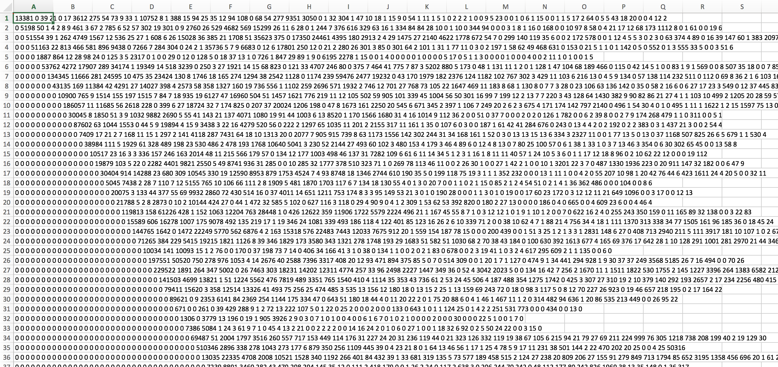
I am a new user to MRtrix and am planning to work on some structural connectome-type analyses. I have performed the HCP tutorial and the resultant .csv file appears to look as follows:
I am wondering if it is meant to look like this where all the numbers are in a single column, not in separate ones as in the screenshot shared by @Alice.
Looks like your spreadsheet software didn’t parse it well: you can still see each row on a separate… row. And each separate number per row is a separate entry (“column”). I’m not sure what software you’re using here, but you may be able to tell it what separators separate elements and rows, and get it imported correctly.
As shown in your .csv file. Does it mean the self-connections(output streamlines that connect to the same node at both ends.) are much more than that connection between the region to regions.
I suspect it is correct? as I guess left Corpus callosum may have a strong connection with right Corpus Callosum.
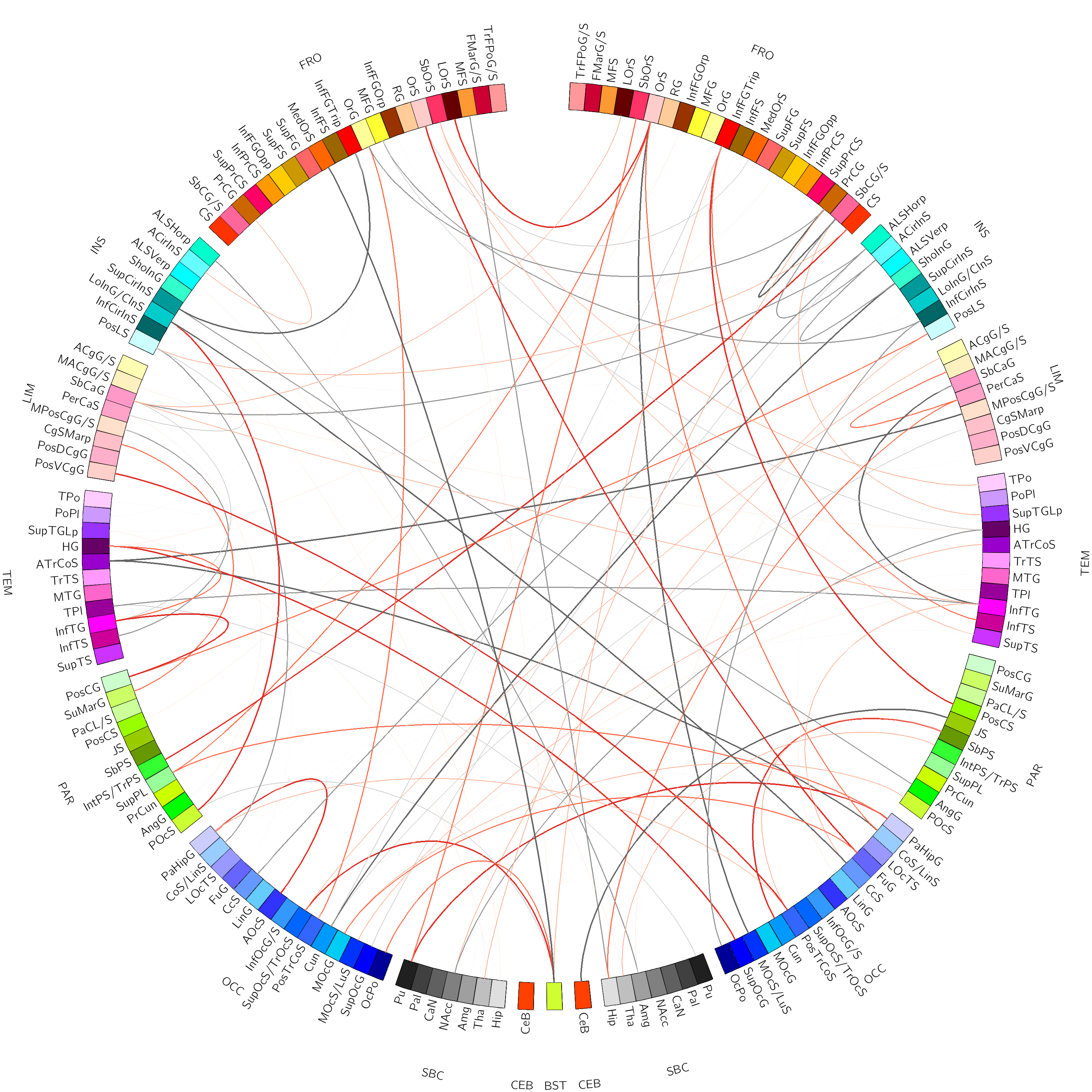
It’s a lot easier (relative to circos) to get the necessary connectomic inputs into the software. Moreover, it nicely details the hierarchical distribution of connections, which can be lost with circos…
Mind you, the connectomes extracted from tck2connectome are asymmetric - meaning you may need to symmetrize them for their use in neuromarvl.


 Let us know!