Hi! I’m exploring the very new ss3t-csd approach on a single subject. I thought it could be useful to share it and have your feedback, so here it goes:
I have single shell (one b0 and 35 b1 volumens) data with low b-value (b1=1000). I applied common pre-processing steps (denoising, unringing, preproc and bias correction) and then I executed the following commands:
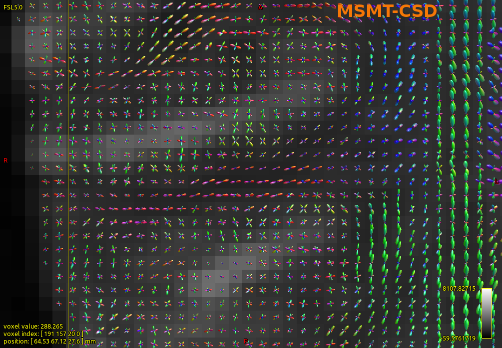
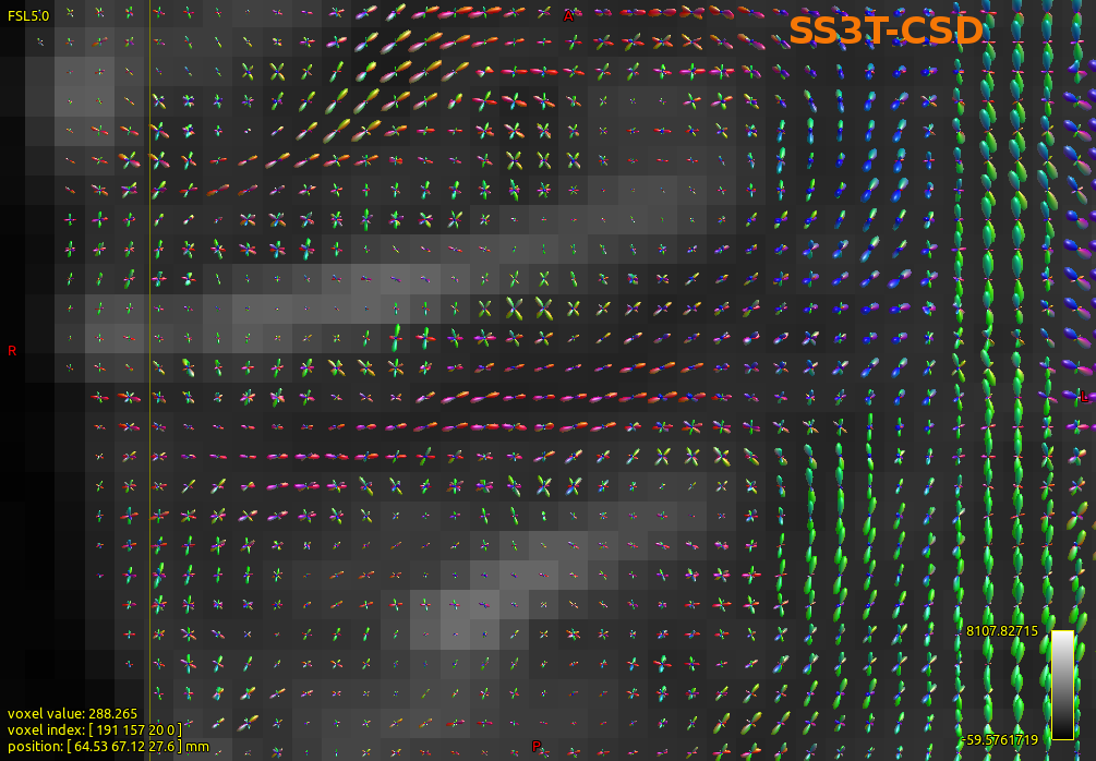
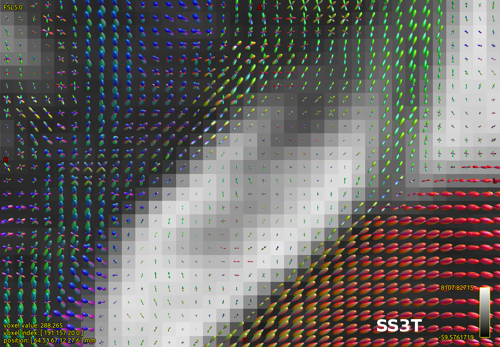
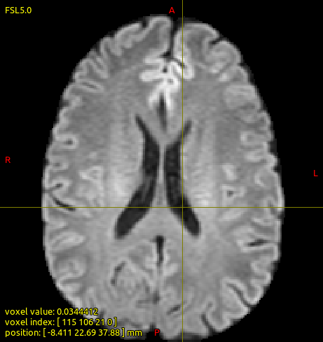
set 2: I wasn’t expecting to find FODs in the CSF area with SS3T-CSD, but they are there. What do you think about that? According to my data, is OK to have FODs in CSF with SS3T approach as well as with MSMT?
That’s very challenging indeed. Worst case SS3T-CSD ends up being “just” 2-tissue CSD, however, I always expect at least some GM to be able to be separated / estimated, so overestimation of WM and CSF (as is the case for 2-tissue CSD) can be reduced.
All good by default.
Looks quite good and reasonable given the limited angular resolution and low b-value. Not bad to get this out of such data still!
Yep, that’s absolutely the aim of the method: by adding a GM compartment, overestimation of WM and CSF compartments in those regions can be reduced or eliminated altogether. It looks like not all overestimation was fully removed (again, due to the limited b-value and low angular resolution), but it’s a step forward. Any reduction of these FOD amplitudes will help e.g. during tractography, as you need to find a reasonable -cutoff value that separates true from false WM.
Yes, I’ve seen that before. This will then always happen equally for 2-tissue or 3-tissue CSD: it’s unrelated to a GM compartment. This is due to all sorts of imperfections in the data leading to still a “range” of diffusivities in those areas. The CSF response function is estimated to fit the largest signal decay or diffusivity. All that is slightly lower in signal decay will need another compartment to kick in. The WM one, especially at such a low b-value, is appealing for the fit because it also allows for anisotropy to fit a little bit of random noise there. That’s what you’re seeing for both methods in those figures. There are some structures in those regions though (e.g. choroid plexus), but they’re normally not anisotropic. The tiny FODs there also show little to no spatial coherence: they can be safely disregarded as noise. SInce these FODs are so tiny, it’s easy to have them separated from all the rest by any threshold value (e.g. -cutoff for tckgen, etc…). So seeing these little (false) FODs is not unexpected; but also not a great worry.
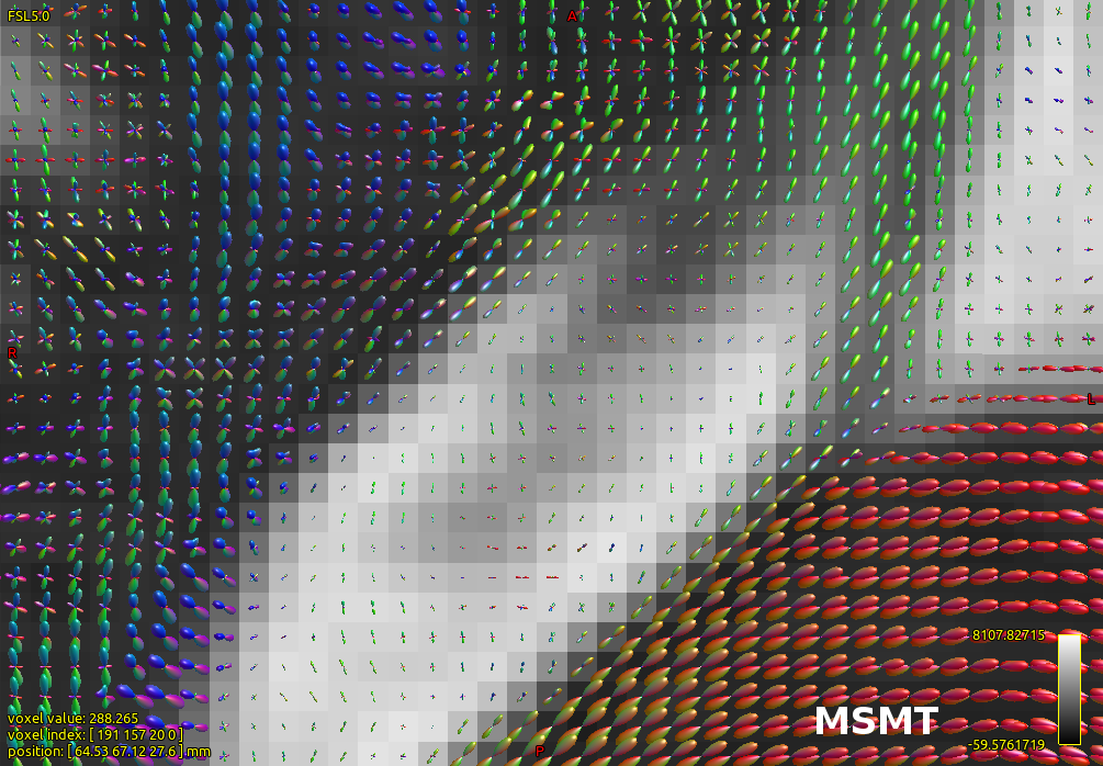
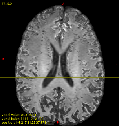
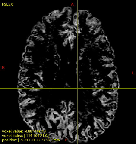
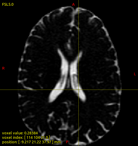
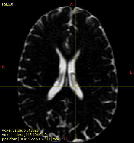
What would be useful to see is all 3 tissue compartments (WM, GM, CSF) you get from SS3T-CSD, and then possible the equivalent 2 tissue compartments (WM, CSF) from MSMT-CSD. You can simply open these up as images in mrview, e.g.:
mrview wmfod_ss3t.mif gm_ss3t.mif csf_ss3t.mif
Make sure to switch interpolation off (as you did in the other screenshots too; e.g. pressing i on your keyboard in mrview); and of course cycle through all images with Page Down or similar.
You’re definitely facing “all” the challenges here: low b-value and low angular resolution, but then also only a single b=0 image. This means a lot depends on that b=0 image, and its exact alignment to all other images. But on the other hand, any improvements you can get e.g. to your FODs are always very welcome at b=1000, I reckon.
Thanks again for giving this a go and taking the time to report!
Thanks for those images! So yes, it’s a balancing act. It’ actually looking still quite good again, given those data! The non-zero WM values in the CSF area are ok, in line with what I mentioned above (same argument) no need to worry there.
The GM compartment was indeed found and has contributed substantially in some areas, as it should. That’s brilliant! The results seem to be better towards the back of the brain, and a bit more challenged towards the front of the brain. I’ve seen results that were better at this particular b-value; so the limitations in your data are (as we already knew before) further imposed by the low angular resolution, and the thing I suspect the most would be the single b=0 image. Even in the 2-tissue result, there’s certain things that are indicating a limitation in the data, leading so some strange things in the contrast (not overly much, but the clues are in there).
I have to say though, at the back of the brain, the result is really surprisingly good for these quality data. In that part of the brain, finding a suitable -cutoff for tckgen should be far easier now, and lead to better results for sure. At the front of the brain, the gains might be slightly less, but whatever you gain is still a win.
Finally, there’s a parameter of SS3T-CSD that you could consider to modify for a scenario like yours (also described here), but I don’t think I would risk to push it here though. As that page also mentions, we simply have to acknowledge the limitations of these data (and be happy with limited gains in any case ).
Start with something like 0.07 or 0.08 maybe; but I reckon the best value might possibly be higher than that for these data. The only way to know is indeed to simply try some values and see what happens. You might also consider running mtnormalise first even; it (should) never hurt(s). If you do that though, the best value for -cutoff will again be different (compared to not having run mtnormalise first).
So in conclusion: given the data, this is looking quite reasonable still. But yes, the data has strong limitations for sure.
In the mean time, just to add to this as a good reference: @archithrajan1 posted some feedback for his b=2000 (single b=0 image) data over here. It’s indeed better than your b=1000 data here (but that’s also fully expected of course). I’ve seen (and tested myself) several b=2000 cases: those are often still very close to “on par” with b=3000 results (not exactly, but very close). At b=1000 though, things start to get far more challenging: all the relevant contrasts in the data start to get far weaker. They’re still there though, and the principles still hold for sure; it’s just much harder to exploit the relevant information when they’re so little contrast.
Thanks for that nice overview; it comes in really handy being able to open all those images in browser tabs and flicking back and forth through them to compare directly (for the same field of view).
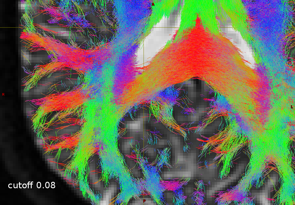
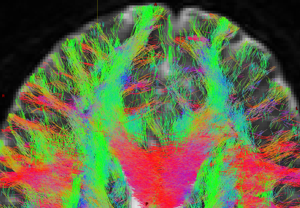
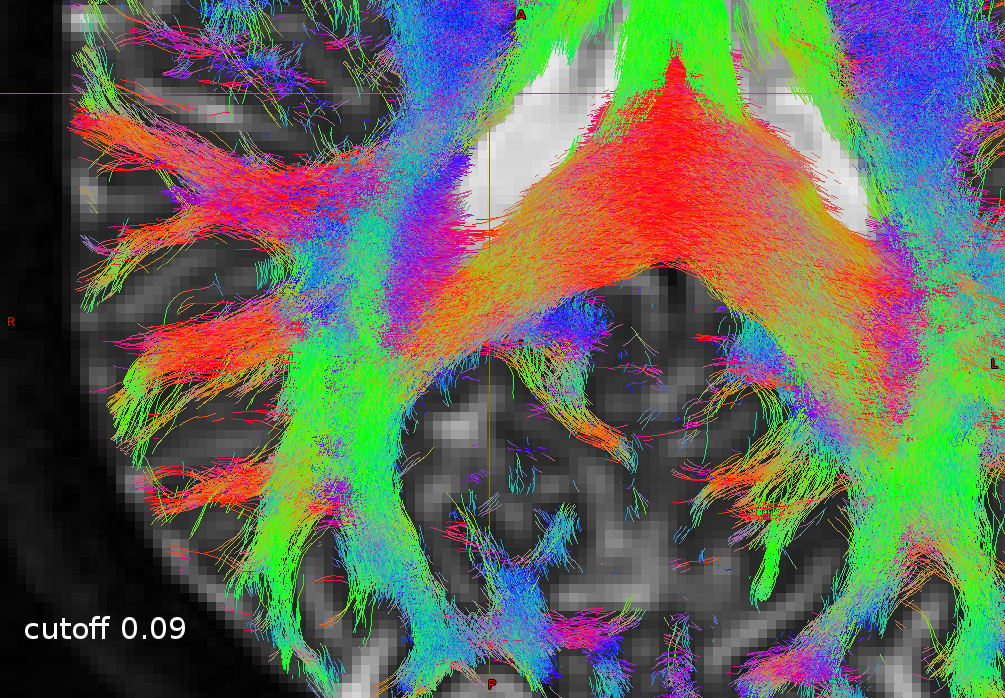
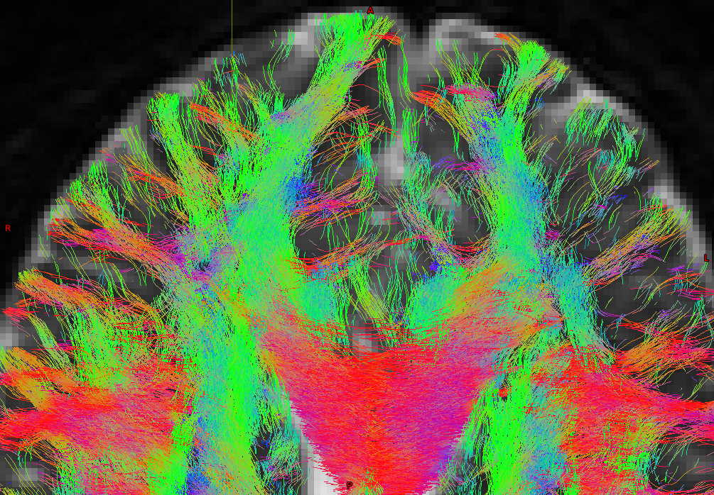
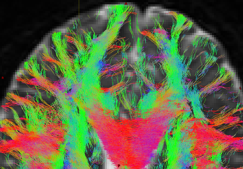
You’ve definitely chosen the right range to explore and display here. This is always hard to judge, but I personally reckon, looking at those images, I’d prefer the cutoff = 0.09 case! In all results, the posterior end of the brain looks actually really good; in general actually, but even more so considering the original acquisition definition. This is always interesting to see: it shows it’s actually hard to judge from the previous images only, how well (or not) the tractography will turn out to be. But so here, it turns out great! The anterior end of the brain reveals just a bit more the limitations of the data quality (just as the previous images did). From what I can see, it seems still quite “safe” to increase the cutoff (e.g. from 0.08) towards 0.09. It cleans up things a bit, and I can’t spot any obvious (within-slice) gaps. At 0.10, I’m starting to see some gaps, or at least some areas revealing things going “towards” having a bit of a gap (also partially due to limited number of streamlines of course, but it does tell us something), in particular in the figure of the frontal end of the brain. So increasing it to 0.10 seems a bit (too) risky to me. 0.09 seems like a nice balance! And again, wow, the posterior end of the brain comes out really well given the data quality.
So given the results in the end here, it looks like you should actually be fine with the defaults on that front. I’m getting other feedback in the meantime that also suggests (also for very limited quality data) the default performs quite well; better than I initially thought it would in fact. This is great news; it should make things easier and less involved for more users. Your feedback and images here are very useful in that regard.
Thanks again!
For future reference, this was documented and further followed up in this “issue” post on the MRtrix3Tissue repository page. The SS3T-CSD instructions will be updated at some point to reflect that the default parameters still work well for low b-values and low angular resolution data.