Good b-value sensitivity parameter for 2shell

I’m surprised it would take 5 minutes to acquire 64 directions with MB4. We can already do that many volumes in 10 minutes without MB, I’d expect this to take less than 3 minutes. What resolution / number of slices are you targeting?

In any case, you’ll probably be able to do 3 shells in 10 minutes with that setup. That will allow you to get >128 volumes, which you can split up in a relatively sensible ratio in the region of 10, 18, 32, 68 volumes for b=0, 700, 1200, 2500 s/mm² (or thereabouts, depending on what b-values you eventually decide to settle on).

One thing I would recommend is to spread these b-values around in the time domain (and orientation domain too if you can) – i.e. don’t acquire all your b=0 together, followed by all your b=700 volumes, etc. This brings benefits in terms of making motion correction easier, makes the sequence more resilient to interruptions, lowers gradient heating, and often allows the scanner to run the sequence faster (depending on the exact implementation) – see this paper for a discussion of these issues.

As I’d stated in that thread, I don’t think the matter is settled as to how many shells are optimal… 2 shells (+b=0) allows you to do multi-tissue CSD with 3 tissue types, but that doesn’t mean that future applications won’t benefit from additional shells (e.g. Fig 10 in this paper). I don’t think this is a question we can honestly answer without speculating…

Same with the issue of which b-values are optimal. This is something we’re looking into, but at this stage, I wouldn’t want to give recommendations, other than just to say that the b-values I suggested above would probably be what I’d go for if I was in your shoes (for a 3-shell setup). For 2-shell setup, I’d probably opt for 10, 30, 70 directions at b=0, 1000, 2500-3000 s/mm² or thereabouts – again based purely on gut feeling rather than any formal definition of optimality…

Finally, on the question of how many directions for a given b-value, the only recommendation I can provide is to ensure that have at least enough to capture (the bulk of) the information content in the signal at that b-value – see this paper for details (it’s a single-shell analysis, but the results do apply to this particular problem).

Thank you very much for this great answer and all the references! This is very helpful!

I did not describe our population, but indeed our population consists of patients with brain insults, so motion robustness is a big criteria for us, as well as the possibility to extend multi-shell to a 4th tissue type such as oedemas as was done in the paper you mentioned.

We will try to implement your 3-shells suggestion, but I’m not sure it is possible to implement a flexible temporal scheme on a standard machine (ours is a Siemers Vida 3T).

Also about the speed of acquisitions, unfortunately it is not possible to acquire different b-values with different directions nor different TEs in the same sequence, so the only way to implement that for our machine would be to acquire different sequences.

Is it possible with MRTRIX3 to do multi-shell analysis from multiple DWI sequences? If so, should we reacquire one set of b=0 for each sequence, or we just acquire the 10 b=0 at the first sequence?

Thank you very much for your clarifications!
Best regards,
Stephen

It should be possible to do this if you can provide a DiffusionVectors.txt file. Check with your Siemens applications engineer – we do this very routinely. It used to require a Research Agreement with Siemens, I’m not sure whether this is still the case. Lots more info on that in this thread – take a look, see if it helps.

Thank you very much! I discussed with our Siemens healthineer and we unfortunately don’t have the required the access to these advanced parameters, but we might in the future after someone in my team do the required training.

So I tried to tweak to get 3-shells, but unfortunately multiband x4 was too noisy, so I reduced to x3, and I settled for b1000 + b2000 (instead of b1000 + b3000) as b3000 was noticeably too noisy on our machine, for a total of 11:45min. Here is the result (single-shell vs multi-shell analysis for the same healthy subject):

I don’t have much experience with multi-shell, but I think it looks fine, right? :slight_smile:

I also looked at the possibility to acquire multiple sequences and concatenate as one multishell sequence prior to analysis, but I found a thread that suggest this would then require a normalization and is thus disadvised:

So for the moment I think we will settle with this setting, which seems quite good and way better than what we had before :slight_smile: Thank you very much!

How did you assess this? Looking at the raw images is not the right way to assess SNR in these types of data. There is very strong contrast in the angular domain, which also implies that most of each image will be very low signal – but crucially, those regions where the DW gradient is close to perpendicular to the fibre direction will have relatively high signal. I’d recommend looking at the estimated fODFs to get a feel for the quality.

Well, there’s nothing overtly wrong here, but I find it’s hard to tell from the tractography output. It’ll depend on all kinds of other factors, like the use of ACT, and the threshold used in tractography, and the specific algorithm used to derive the fODF (which I assume was different between the single and multi-shell analyses you’re showing?).

Well, it makes things a bit more complicated, but nothing that can’t be dealt with reasonably easily. You just need to be aware of it and make sure you deal with it appropriately. The new functionality in mrhistmatch was added to deal with precisely this issue.

Also, on a Siemens scanner, you can turn off all the adjustments that would lead to scaling differences – see this post in the thread you mentioned. This means that you can avoid these issues altogether, and concatenate the data without worrying about scaling differences. The trick here though is to make sure that only the first scan is calibrated, with all adjustments turned off for subsequent scans.

Thank you very much for your fast reply!

I am going to try to do multiple single-shell sequences and then concatenate into one multi-shell, I guess I can use mrcat to do this (by first extracting the b-0 and b-xxxx values separately using dwiextract)?

About avoiding the calibration for subsequent scans except the first, yes we can do that :slight_smile: But is it ok if then the scans have different TEs? Indeed, I think the only way we can get a benefit in speed is either to reduce the number of angles or the TE for each scan depending on the b-value, but I’m wondering if changing the TE wouldn’t require a recalibration or is it ok?

About data quality, yes you’re right we were using ACT for the single-shell analysis! I remade quickly a pipeline to do single-shell analysis without ACT (sourcecode here), with the same parameters as multi-shell without ACT (sourcecode here). Here are the results:

The only difference between the single-shell and multi-shell is as you guessed the algorithms: dwi2response dhollander and dwi2fod msmt_csd for multi-shell, dwi2response tournier and dwi2fod csd for single-shell. From this picture, it looks like multi-shell is enhancing the results compared to single-shell, no? :slight_smile:

About b-3000 noise, yes indeed I saw a lot of noise in the source image but I know this produces more noise, however the tractography also contain artifacts:

(Notice the small spurious tracts at the bottom of the trunk tracts. Note also a similar artifact was reproduced on another subject acquired at b-3000).

This was done without ACT, so one can argue that using ACT we could remove this. So from this I guessed that b-3000 was too noisy on our machine and b-2000 was better, but you have more experience so what do you suggest? To keep b-3000 and remove the spurious tracts with ACT or stick to b-2000?

Thank you very much again for all your very helpful guidance! :smiley:

If you’re sure the calibration is identical between scans, you can just mrcat them together – no need to use dwiextract at all. The DW encoding will contain all the information about which scans used which b-values.

Even if you do need to correct for different scaling between acquisitions, there should still be no need to use dwiextract when combining the data.

No, not in general. Most analysis algorithms will assume the exact same acquisition parameters have been used throughout. Interestingly, MSMT-CSD is probably the only method I know of that should be able to handle these types of data, but I’ve not seen anyone do it yet. I’d strongly recommend you use the same TE for all acquisitions you wish to combine, it’ll make your life a lot easier later on, when you come to publish, etc.

The main reason to split your acquisition into separate scans is to allow different numbers of directions per shell. I agree that in theory you could also reduce the TE to boost SNR and reduce acquisition time further, but like I said earlier, it’s not a good idea since it breaks the assumptions of almost all analysis methods you might like to use (outside of MSMT-CSD).

Yes, that’s much more in line with what I was expecting. It’s still not comparing like with like though… :wink:

The dwi2fod csd algorithm produces slightly different outputs than the dwi2fod msmt_csd algorithm, even when set to the same parameters. This is due to the use of a soft non-negativity constraint in the csd variant, as opposed to a hard constraint in msmt_csdsome discussion on this issue here. If you’re really keen on performing a proper head-to-head comparison, you could use the dwi2response dhollander and dwi2fod msmt_csd algorithms for the single-shell analysis also, but only provide WM and CSF responses (and corresponding output files) to the dwi2fod msmt_csd call – as per the same thread.

I assume you’re referring to the cluster of spurious streamlines next to the spinal cord / cortico-spinal tract? That’s most likely simply down to poor masking… I’d expect it would be entirely dealt with using ACT. I certainly wouldn’t take any account of it to assess the quality of the reconstruction, you really need to look at the results within the brain, and preferably in the central deep GM regions / brainstem, where the SNR is typically lowest (furthest from the coils).

Like I said earlier, looking at whole brain tractography as a marker of quality is fraught with difficulties (it annoys me when I see these types of comparisons used as ‘validation’ in papers…). So it’s difficult for me to make any meaningful statement on the quality of your results from what you show. I’d personally use other strategies: you could compare the raw fODFs within the central brain regions, and maybe compare the slab-cropped whole-brain tractography in those regions. But personally, I tend to look at the SNR in the b=0 images, assessed as the voxel-wise standard deviation over repeat b=0 volumes (don’t let it drop too far below 20), inspect the quality of the DW encoding (dirstat provides a lot of information on that front), check that the fODFs look as expected, and verify that there are no obvious artefacts (due to e.g. incomplete fat saturation, ghosting, residual eddy-currents problems, etc). The decision as to which b-value to use should probably be guided by other considerations, but these days I’d advocate somewhere between 2,500 to 3000 s/mm² for the highest shell.

Really, this depends on what you hope to do with the data, and future methods will undoubtedly come up that might require higher b-values, etc. It’s really hard to provide any definitive recommendations for a future-proof acquisition, or even for an optimal acquisition for current methods, there are so many things that can be done with these data, and what’s optimal for one type of analysis may not be for another, etc…

Thank you very much @jdtournier for your very wise and well explained advices. I implemented the changes but could not comment about them until now (holidays break, no subject to acquire!).

So I tried to do additional quality checks as you advised, however I could not do them all as it seems most rely on experience to interpret, which I lack on this modality. So far, I checked the tractography, the fODFs, the raw b=0 and b=xxx volumes to check for any artefact and general noise, and this guided me in setting the current parameters. After learning a bit more about the theory and given your advices, I headed towards 3shells, as this can potentially allow to extract lesional matter with CNSF as you referenced.

In the end, I finally settled for 3shells DTI in separate sequences without recalibration, using “Copy Reference” with “Adjustment” checked (Siemens machine) - I think this how the “no recalibration” is done on such machines?
More specifically, we now have a shell with b700 30dir, one shell b1000 64dir high quality (low TE = 89ms), and one shell b2000 64 dir with a higher TE (to allow for lower TR and TA - acquiring higher b-values seems to take a lot more time). Although you advised not to use different TEs, this is unfortunately the only way we can afford to do 3shells in a reasonable timeframe (~13min), the other solution being to use only 2 shells. I hope future methods will be able to account for that, but for the moment it seems we can get reasonable results with the current implementation of msmt_csd, as you said it seems to account correctly for different TEs (as I cannot notice much difference with different or same TEs when using 2shells).

For reference, the sourcecode I used during this discussion is here and I uploaded here the PDF of the protocol of DWI sequences we implemented (beware, the printout does not include “Copy Reference” with “Adjustment”, but this must be done in the Dot Cockpit interface).

(BTW it would be nice to be able to upload PDF files here, would help sharing the protocols :wink: )

I’ve just enabled upload of PDF documents (it’s disabled by default due to security concerns).

Thanks for feeding back on your progress otherwise. Hope it all works out OK!

Just to say that after trying on more controls and also patients with brain damages, everything looks to run very fine! The tractographies look very good and a lot more detailed than what we had before (in particular the cerebellum, which was lost with ACT most of the time!).

We are now looking into the possibility to use a RESOLVE sequence (Siemens, synonym of readout-segmented multi-shot EPI) instead to increase the resolution and quality, but otherwise it works already very well.

As an illustration of what you said before (that the raw images noise does not necessarily reflect the DWI quality), here is a comparison of the raw images and Colored Fractional Anisotropy (ColFA) for multiple b-values. Although the raw images seem noisier with higher b-values, the ColFA seem on the contrary to be less noisy and more precise:

1 Like

Hi-
We’re working on setting up a 2 shell acquisition on our new Prisma to be used primarily for tractography on chronic stroke survivors and older controls, and running into some issues somewhat related to this thread.
First, we’ve run into a lot of problems with exceeding SAR limits when using multibanding. Is this common? I haven’t seen any discussion of this issue, but it took a few hours for us to find parameters that the scanner would even run, and I think we’re still pushing the upper limit of what our scanner will allow. We could always break our scan into two parts if needed, but I don’t think we’re doing anything outlandish that should require that.
Ultimately, here’s what we got to run (which is very close to what we wanted anyway):
2mm voxels
7 volumes at b=0, 40 at b=1200, 80 at b=3000-- we’re using Emmanuel Caruyer’s script for getting the vectors and inserting b=0 images interspersed throughout
SMS at 2, GRAPPA/iPAT off
Partial Fourier at 6/8
TR=4700
TE around 85
acquisition time 10:30
We also tried it with TR of 6000 because my understanding is that longer TR = better SNR, although I don’t know if it’s worth the extra 2.5 min given we’re trying to squeeze a lot into one session.
We’re figuring out how to do the QC now-- to the eye the b=0 images look really nice, but there’s some obvious ghosting on the b=1200 and b=3000 images. Is there a typical cause of this in the acquisition parameters that we could adjust?
Any other advise on setting up a high quality sequence along these lines (without nuking our patients) would be greatly appreciated.
Thanks!
Peter

The experts of MRTRIX might provide a more enlightened answer, but I can tell you what we experienced with our new protocol.

SAR was indeed increased and we have a warning, but it’s not exceeding the safe limit (the machine still allows to run the sequence). So we systematically bypass this message (this was validated in situ by a Siemens Healthineer). This indeed happens only with DWI (we also use multiband with similar parameters for BOLD and we have no SAR warning). You can also have a look at the type of gradient used (normal, fast, etc) and the bandwidth, by playing with these you can reduce the SAR (at the expense of total acquisition time or quality).

About the quality, from my experience having a low TE matters more than having a low TR. I did not notice a particular difference when using a low TR, but I did when using a low TE vs a high TE. In our protocol, we use the lowest TR possible to speed up acquisition, but we try to maintain a low enough TE for sufficient quality.

Hope this can help,
Best regards,
Stephen

Dear experts,

we are currently setting-up a new DWI protocol for our new Siemens Vida 3T scanner.

  • Purposes: CSD-based tractography, structural connectivity, FBA
  • Aim: best possible angular and spatial resolution
  • DWI measurement time plan: approx 15 minutes
  • Multiband at the disposal.

Based on discussions on this forum and recommendations in publications, especially

we tried to set following DWI scheme on our product DWI sequence using custom diffusion directions:

gen_scheme 2 0 12 1000 40 3000 160

i.e. diffusion scheme split to 2 separate series with opposite phase encoding direction (AP/PA).

The aim was to dedicate most possible time to gain SNR on b=3000. b=1000 (instead of something around b=1500) was selected due to retain ability to fit diffusion tensor model on the data, if needed.

Main measurement parameters:
MB factor 3, voxel size 2x2x2 mm3, 69 slices, TR=4500 ms, acquisition duration 2x8.7 minutes.

To assess the quality of the data and SNR requirements using selected voxel size, I tried to evaluate SNR of b=0 and b=3000 shell.
I read recommendations not to go below SNR = 15 in b=0 shell by @jdtournier
and aim for SNR>5 in most outer shell by @dchristiaens (althought, he, admits, it is difficult to achieve).

I am using following commands to get SNR, partially adapted from this thread:

dwidenoise dwi.mif dwi_denoised_extent_7.mif -extent 7x7x7 -noise noise_extent_7.mif
dwi2mask dwi_denoised.mif mask.mif

Concerning noise estimation, I found two recommendations:

  1. using voxel-wise std of b=0
dwiextract -shell 0 dwi_concat_denoised_extent_7.mif - | mrmath - std -axis 3 - | mrstats -
      volume       mean     median      stdev        min        max      count
       [ 0 ]    15.1416 5.64851093    27.0527          0    785.402     690000
  1. using estimated std of noise from dwidenoise
mrstats -output mean -mask mask.mif noise_extent_7.mif
10.6097

The results are quite different…

Signal in shells:

dwiextract -shell 0 dwi_concat_denoised_extent_7.mif - | mrstats -output mean -mask mask.mif -allvolumes -
223.168
dwiextract -shell 1000 dwi_concat_denoised_extent_7.mif - | mrstats -output mean -mask mask.mif -allvolumes -
78.423
dwiextract -shell 3000 dwi_concat_denoised_extent_7.mif - | mrstats -output mean -mask mask.mif -allvolumes -
33.7226

Thus, SNR, using method 1 in shells is
b=0: 14.7
b=1000: 5.2
b=3000: 2.22
usind method 2
b=0: 21
b=1000: 7.4
b=3000: 3.1

Could you please comment on on our prepared protocol?

  • Is the SNR, in your opinion, sufficient? SNR>5 condition in outer shell is not fullfilled. Should we rather increase voxel size to get better trade-off between SNR and angular/spatial resolution?

  • Is the rather large amount of directions for b=3000 beneficial to gain SNR, regarding possible pitfall with rician bias on low SNR, as mentioned in following thread?
    SNR calculation comparable to dipy? - #5 by jdtournier
    Or should we rather spend acquisition time by acquiring additional b shell? I was considering to add the shell to be able to model additional compartment as mentioned here:
    Good b-value sensitivity parameter for 2shell - #2 by jdtournier

  • What method, from the listed two, do you recommend for noise estimation, seeing the fact that each produces different result?

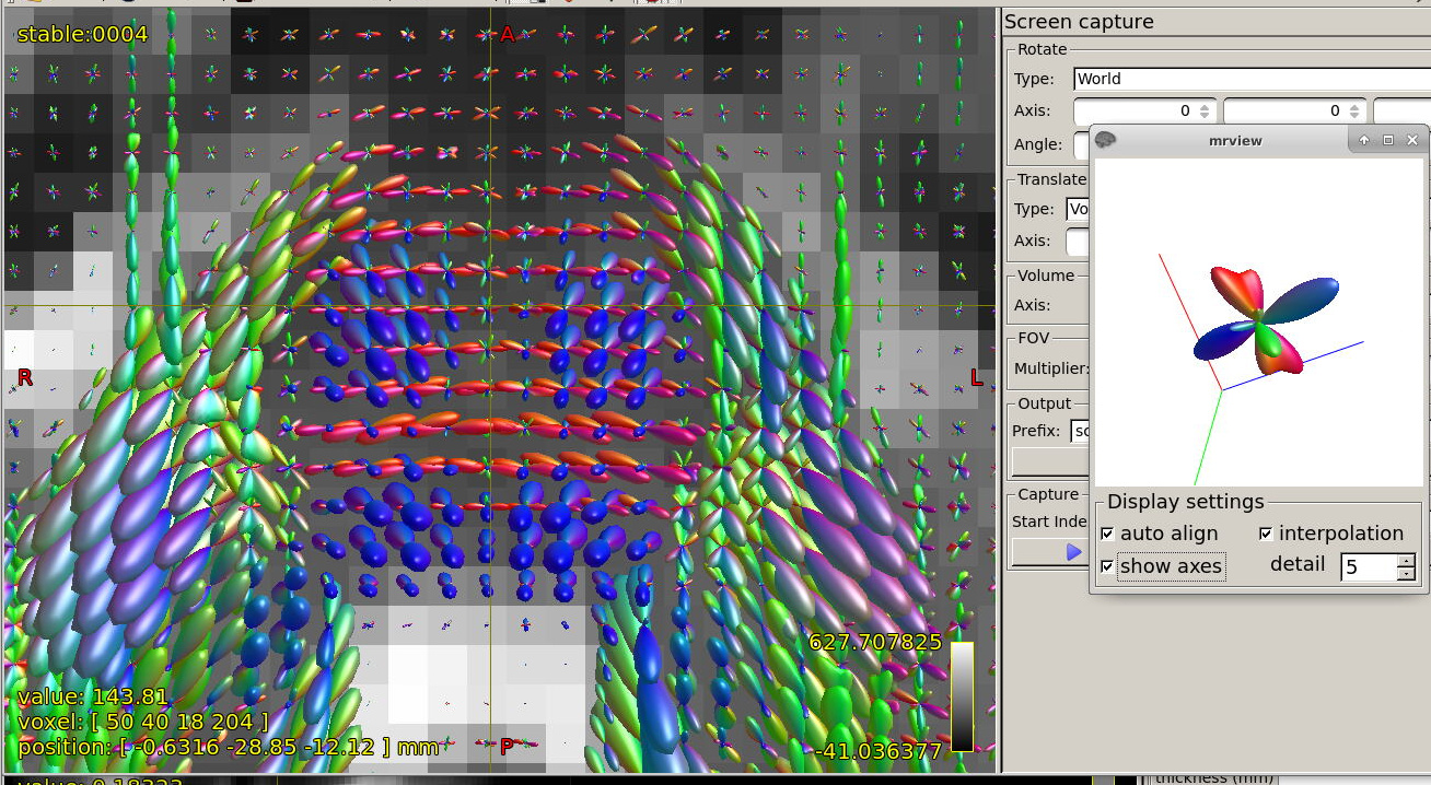
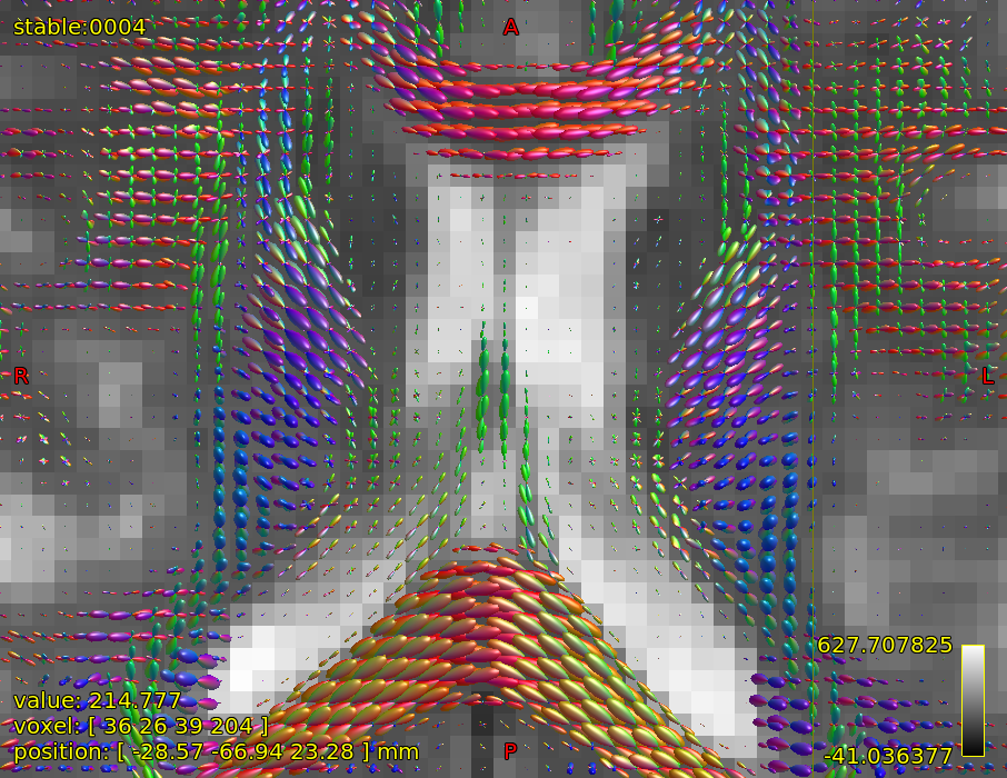
Further recommendation was on optical inspection of fibre responses and ODFs. I am sending several screenshots of their estimation on our testing data. Could you please look at them to asses whether the protocol is tuned reasonably?

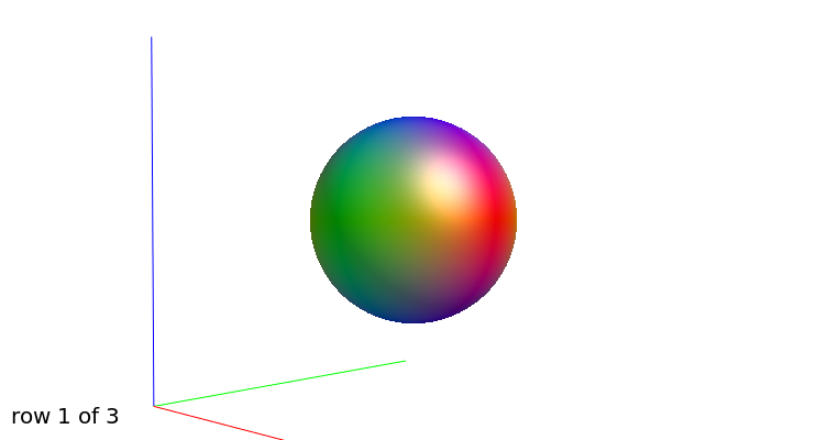
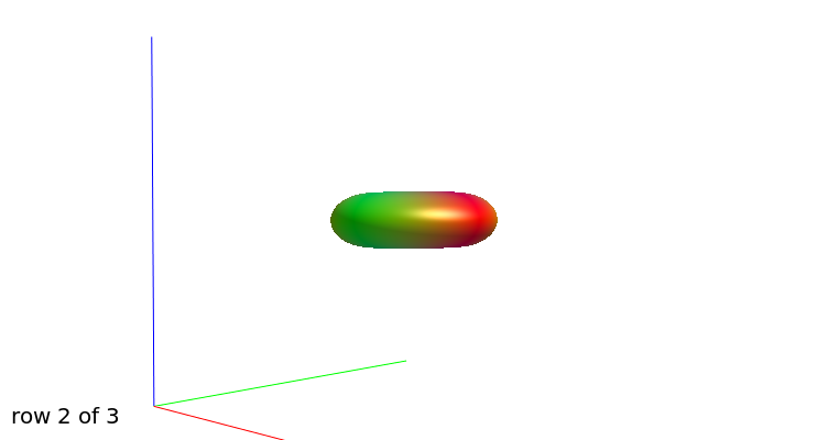
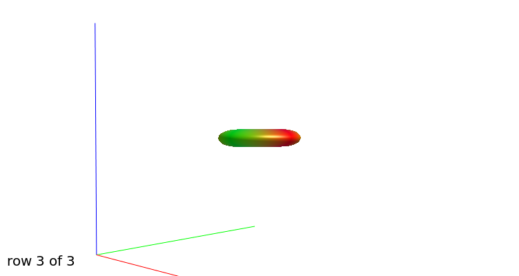
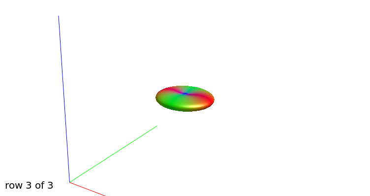
WM response functions:
b=0


b=1000

b=3000

b=3000, another view

FODs in brain stem in region of cerebellar penduncles:


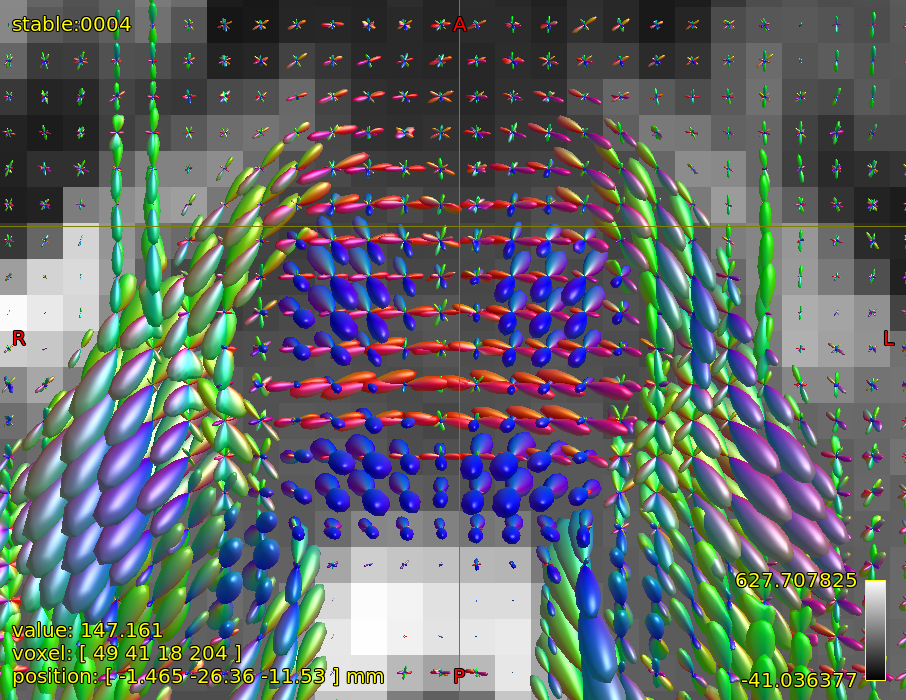
The FOD inspection at focus is showing quite complex shape, at least 3 fibre directions, could it be trusted?


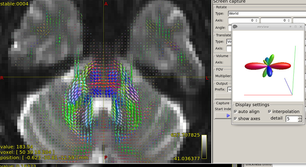
FODs around ventricles:

Could you please comment on? Is this protocol efficiently optimized?

Last questions concerning data acquisition/post-processing:
Do you have experience with the option “dynamic field correction”? I think that it is better NOT to use this, since this correction would be done more efficiently by eddy.
Do you use option to re-scan image when data corruption/image artifact is detected during scan?
Do you use some data filtering on the scanner (image filter)?

Considering post-processing: Would you recommend some upsampling to “gain” spatial resolution?

Thank you very much in advance for your suggestions/comments.

Antonin

OK, that’s a huge (set of) questions… I’ll try to answer as best I can. First off though, the usual caveat: much of this is subjective opinion, I don’t think there is such a thing as an ‘optimal’ acquisition without defining very precisely what it is you will be using it for, and what your constraints are (you can always improve your acquisition by spending more time, for instance). That said, I think we generally all agree on what a ‘good’ acquisition is, and even more so on what a ‘bad’ acquisition looks like…

In general, I think your decisions look very reasonable, and the protocol as a whole seems pretty solid to me. Your responses and FODs look very reasonable and clean to me.


On the SNR calculation issue, a few points:

  • the dwidenoise -noise output provides a map of the estimated pure Gaussian noise. Anything that doesn’t look like pure thermal noise will not be considered as noise, and that includes physiological noise like signal dropouts and instabilities due to motion and other processes. In many ways, it’s the lower bound for the noise in your signal.

  • the standard deviation of the b=0 volumes is probably more reflective of the genuine signal variations in your data, due to thermal noise or other issues. However, you’ll find that this measure is often greater in the b=0 images than the DWI volumes in the CSF (there seems to be quite a bit of instability in the CSF signal for some reason, probably due to CSF pulsation or flow). So that measure is OK as long as you don’t include CSF regions in your estimate.

  • On modern multi-channel systems, the SNR is spatially variable. While a single summary variable might be informative as an overall benchmark, you should at least restrict it to those parts of the brain you’re interested in, most likely the white matter. Using a whole-brain mask will bring in the CSF, which can be problematic. You can improve things by measuring the noise and signal from a crude white matter mask, e.g. thresholding the power in the l=2 SH fit to your highest shell using:

    dwiextract dwi.mif -no_bzero -singleshell - | amp2sh - - | sh2power - -spectrum - | mrconvert - -coord 3 1 - | mrthreshold - wm_mask.mif
    

    and taking the ratio of the mean or median signal within that mask in the b=0 image to the mean or median noise level within that mask.

    Better yet, generate the SNR map by simply dividing your mean b=0 image by your noise estimate, and check the values in the most problematic relevant regions. That map will probably be quite noisy, so you can also filter it with mrfilter smooth or mrfilter median. You’ll typically find that the SNR will be lowest in the brainstem, so you may want to ensure you have adequate SNR in that region, which will also mean higher SNR elsewhere.


Looking at your data in particular, your SNR seems a bit low for a 2x2x2mm acquisition. I note that you’re also using the denoised data to compute the standard deviation of the b=0…? So if anything, that value would be an overestimate of the true standard deviation if it were computed from the non-denoised data…?

In answer to more specific questions:

Yes, I think it looks sufficient, but I would try to get a better handle on what your SNR actually is, as mentioned above. In my experience, shooting for SNR>5 in the outer shell requires compromising quite heavily on resolution, and this amount of SNR would in my opinion only be required for more complex microstructure modelling.

This is difficult to judge from the information presented. Ultimately, I recommend you try acquiring a few datasets at slightly different resolutions, process them, and have a look at the quality of the reconstructions you get, in the context of what you want to do with them…

Yes, I think so – provided your SNR is not too low, as per the recommendations above. You can also do quite a bit to avoid the Rician bias if you can acquire the complex DWI data (see below).

That is again dependent on what you want to do… Our current ‘default’ pipelines only require 3 distinct b-values (b=0 + 2 shells), but things will no doubt evolve over time. Personally, I think if you’re setting up a relatively future-proof protocol that you intend to be used for multiple studies for the foreseeable future, you’d be well advised to acquire an additional shell if you can…

I think both have some value, as long as you understand what each is reporting on. Personally, I think the std(b=0) is probably more useful as it captures more sources of variation. There’s also other ways to estimating noise from the DWI using e.g. adjusted residuals from a SH fit, and that’s what I might often use myself. But the standard deviation in the b=0 is I think the most widely used, is easiest to explain and the least controversial…

I’m not sure what this one does… Is this correcting for frequency drift during the acquisition…? It might be worth doing if you notice signal drift over the course of your acquisition, but I can’t say I have much experience here.

We do for the dHCP, but that’s a very unusual cohort, and requires a very bespoke acquisition sequence… This is not usually an option using standard sequences – unless this is a new feature I’ve not come across yet.

I would avoid these, since they’ll no doubt entail some loss of resolution, and the Gibbs ringing can more effectively be removed using mregibbs.

There is some evidence that it might help, but I must admit this is not something I ever do…

Final point: if you can get your scanner to output the full complex images (i.e. phase in addition to magnitude), it’s very much worth doing. Denoising on the complex data vastly improves the performance of the denoising (see e.g. this paper), because it means the noise is actually Gaussian (not Rician), which better matches the MP-PCA algorithm’s assumptions, and by denoising in the complex domain, your subsequent magnitude images have vastly reduced Rician bias.

1 Like

I’m trying to address some of the same questions myself at the moment; unfortunately there are too many knobs and no objective criteria…

gen_scheme 2 0 12 1000 40 3000 160

gen_scheme (specifically the dirmerge step at the end) is designed for systems where the phase encoding direction can be altered on a per-volume basis during a single protocol, which isn’t possible for Siemens. So I’m not sure whether the hierarchy of logic is optimal. I’ve been using this: it does mean that e.g. the eddy current optimisation is done independently per shell which isn’t ideal, but it exports directly to DVS which is convenient.

Do you have experience with the option “dynamic field correction”? I think that it is better NOT to use this, since this correction would be done more efficiently by eddy .

I don’t actually recall exactly what this setting does, I’d need to consult the documentation.

Do you use option to re-scan image when data corruption/image artifact is detected during scan?

This is actually more difficult now than it used to be because slice-to-volume motion correction and outlier detection / replacement can make data historically considered too corrupt entirely reasonable.

Do you use some data filtering on the scanner (image filter)?

Absolutely disable these; they will actually interfere with mrdegibbs.

Will the denoising of complex data, using the algorithm in the link you posted, be part of the next version of MRtrix?

Good question. First off, It’s already possible to do it, but it requires massaging your data a little bit first, to convert it to real & imaginary (as it often comes off the scanner as magnitude & phase), with real and imaginary as separate volumes (so you end up with twice the number of volumes), denoise that, and finally compute magnitude of the output. Nothing complicated, but fiddly. It’s also going to depend on how your scanner presents the data, which is part of the reason we’re not sure how best to support this.

But we have discussed the possibility of supporting actual complex input data (i.e. with a explicit complex data type). That part should be easy (might even be in dev, @dchristiaens?).

Direct denoising of complex input data (as CFloat32 or CFloat64 data types) is supported on dev and will hence be part of the upcoming release. As Donald already mentioned this can have a major impact, especially in low-SNR data, because it reduces Rician bias in the data.

However, this implementation is still a “light” version of the cited paper. It supports complex input data and also includes the improved noise estimator, both of which are major improvements, but does not (yet) demodulate the phase and does not account for spatial noise correlations in parallel imaging. The former is easy to do in matlab/python/… and could be added to MRtrix at some point. The latter can only be done with access to the MR reconstruction process and is therefore not something we will support anytime soon.

This is nice, however, neither our product multiband DWI sequence on Siemens Vida, nor DWI multiband sequence from CMRR (Minnesota) on Prisma does not support storage of complex data, unfortunately :frowning: This would preclude the use of this option for most common users, I reckon.

DWI multiband sequence from CMRR (Minnesota) on Prisma does not support storage of complex data

Are you sure? I’m doing this on our Prisma here. It’s a very general setting in the protocol editor that exists at a lower level than the particulars of any specific sequence. You need to change “Reconstruction” to “Magnitude and phase”, and then convert the resulting two DICOM series to native complex data using mrcalc, specifically scaling the phase data to Radians and then using the -polar option that was added to the dev branch in #1659.