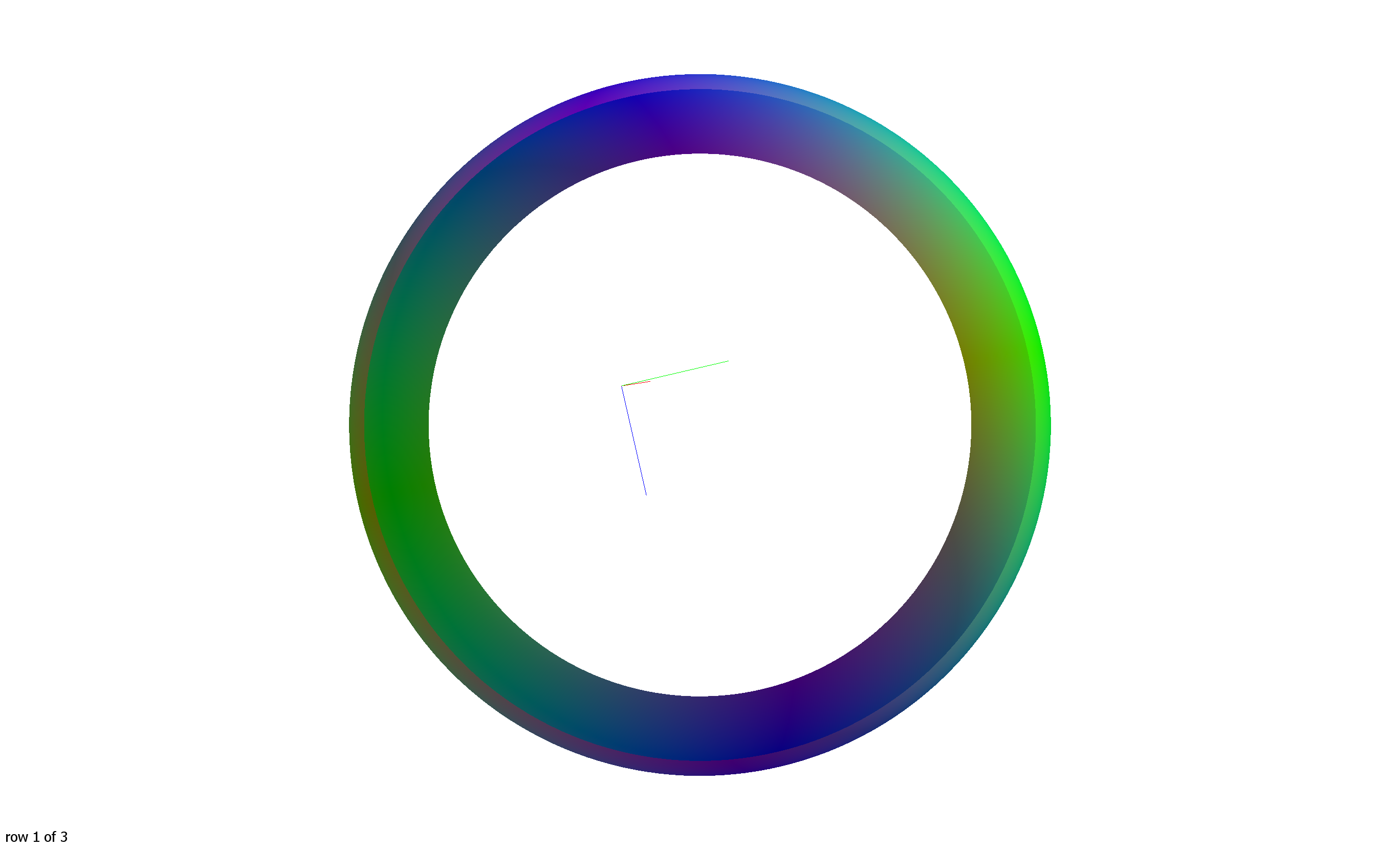
What parameters should I consider to adjust in order to improve the response function estimation when processing a 0.7 mm iso diffusion dataset obtained with b=0, 1000, and 2000 s/mm2? I applied dwi2response dhollander with default parameters, but to find 1) a bump in the estimated response function for WM and b= 2000 (see first figure attached), 2) that the estimated response function for CSF and b=0 shows up in shview as a big ring (instead of a ball) (see second figure attached). Other response functions estimated however looked reasonable. Any advice on improving this?
There’s a good chance your responses are entirely appropriate…
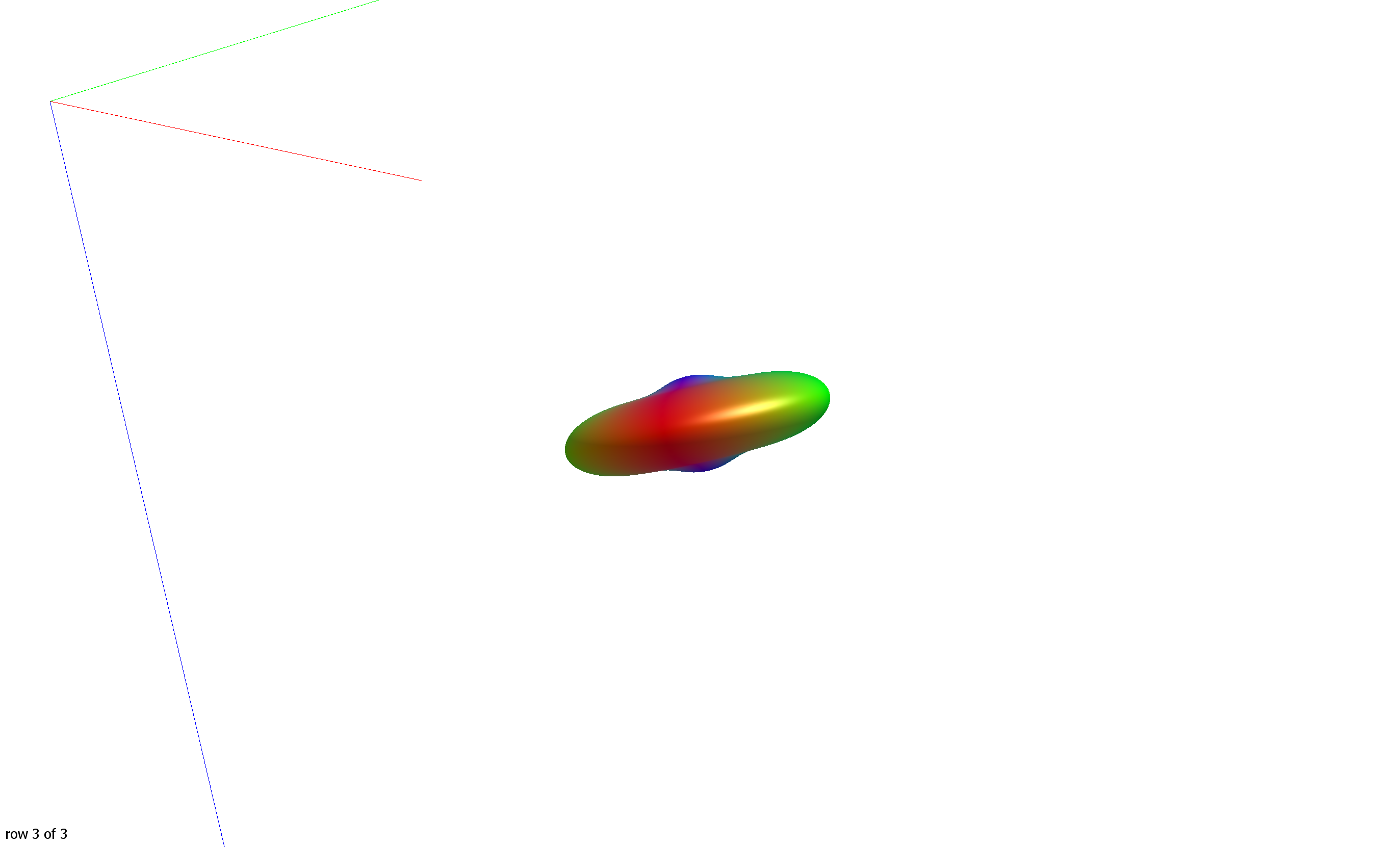
For the WM response, the bump you’re seeing is not uncommon, and most likely caused by the Rician noise bias that you get with magnitude data. This would not be unexpected in a high-res sequence, which is presumably very noisy. There’s a good chance it won’t affect your analyses too badly. But if you really want to get rid of it, you’ll need to figure a way to reduce or minimise the Rician bias in your data. In my experience, this is easier said than done… But there are approaches out there, depending on your data. The best approach in my opinion relies on having access to the raw complex data, before any magnitude transformation (or averaging, which makes the issue worse): it consists of removing the relatively smooth phase variations in the images, before discarding the imaginary component, which at this point should be just noise, and using the real component as the signal, which at this point should still have Gaussian-distributed noise.
For the CSF response, this is likely due to scaling of the display. Try hitting the Escape key to re-scale. The reason you’re seeing what you’re showing is that in OpenGL, we have to define the viewport, including near and far planes. Any points outside this range are simply ignored. So what you’re seeing are the regions of a (large) sphere that lie between the near & far planes. I can’t remember exactly what I’d set these to, but from memory it’s 5x the size of the axes. But like I said, simply hitting the Escape should reset the scaling to something sensible…
Yep, judging from what’s shown, I can only agree with that (for the same reasons). Note the “bump” is merely an illusion of the (3D) radial plot: the response function shown is still monotinically decreasing from maximum to minimum amplitude (you can even visually tell, because the bump is “flatter” than the curvature (well, eccentricity) of a sphere).
Apart from @jdtournier’s point about SNR at that spatial resolution, I’m just wondering: what’s the “subject” here? Is this in-vivo data? Should it be ex-vivo, that would be another explanation: in that case, these b-values are “quite low”.
Thanks for your comments.
These data were in vivo human brain diffusion at 7T. Did you mean if I could acquire the data with higher bvalues, I would probably reduce the chance of having the bumps in the estimated response function?
BTW: Another dataset acquired in the same volunteer with the same b values, but at lower resolutions (1.05 mm iso), did not present the bumps in the estimated response function for WM and b=2000.
xiaoping
Aha, 7T, the final piece of the puzzle. Now I get where the high resolution is coming from indeed.
So yes, in this scenario (same volunteer, same b-values, but different spatial resolutions) @jdtournier’s explanation is the one you’re looking for: the SNR will be lower in the higher spatial resolution dataset, resulting in a stronger Rician bias; so the “bump” (even though not really a bump!) is the noise floor here.
Don’t worry about it though, these small bumps barely affect the CSD outcome in any important ways: much more important is the rest of the “shape” (contrast) of the WM response. It’s again a bit of a problem of the radial plot visualisation, which makes us focus on the “bump” as destroying the “disc” we’re looking for; however, much of the shape of that “disc” is in the high amplitudes (whereas the bump-or-no-bump thing is only a feature in the tiniest of amplitudes of the WM response function).