Neonatal multi-shell data: optimal preprocessing

mblesac · July 11, 2019, 10:45am

My framework has changed quite a bit, I was using fdt_rotate_bvecs from FSL. Now, I don’t use any special command to rotate the bvecs, eddy does it everything internally.

I have three acquisitions in the same session, one shell of bvalue 750, one of 2500 and one with 3 reverse encoded B0. Briefly speaking what I do is:

-Inspect the data, and if the first B0 of the 750 shell is affected by any artifact, change it by the next B0 that is not affected by any artifact. This is very important for this data, because the movement is very big with the babies, and if you feed corrupted images to topup and eddy, they will probably crash

Concatenate the 750 shell and the 2500 shell (also the bvecs and bvals).
Concatenate the first B0 of the 750 shell with the first good B0 of the reverse encoded acquisition.
Denoise the concatenated data (dwidenoise).
Run topup to estimate the field.
Run applytopup to the denoised data.
Create the mask of the average of the B0 of the corrected data (bet).
Run eddy to the denoised data (with --repol and --mporder flags). This command will correct all the bvecs
Finally, run dwibiascorrect to correct for bias field inhomogeneities.

That’s pretty much everything from the diffusion side, note you can add mrdegibbs to the pipeline, I didn’t do it because my data is partial fourier acquired, and just to be extra safe, but there are some posts suggesting that you can run it as well in partial fourier acquisitions. Also several of this steps you could do it using mrtrix scripts, but I like to work with the steps separated.

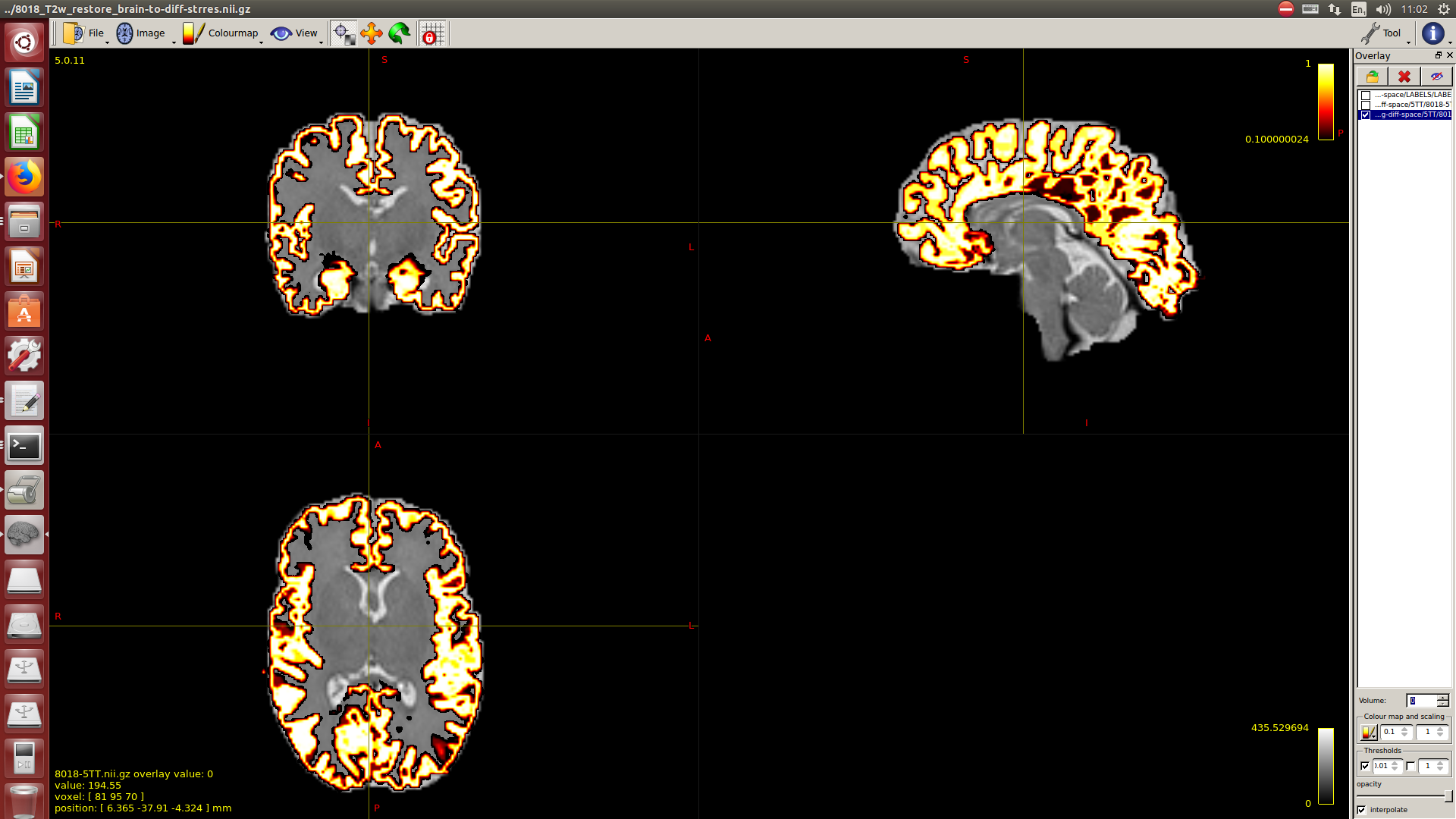
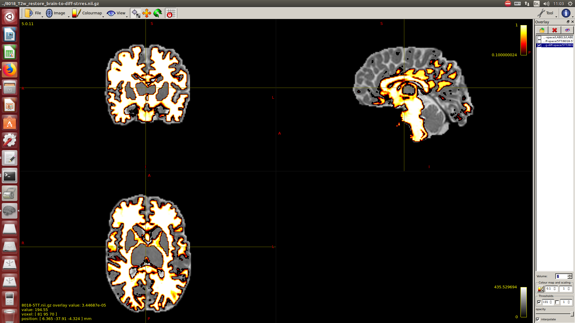
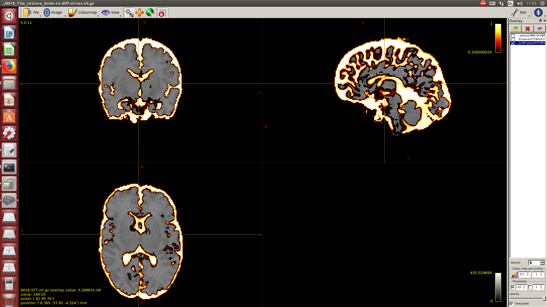
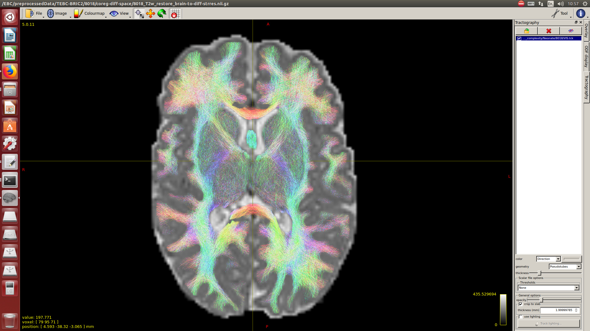
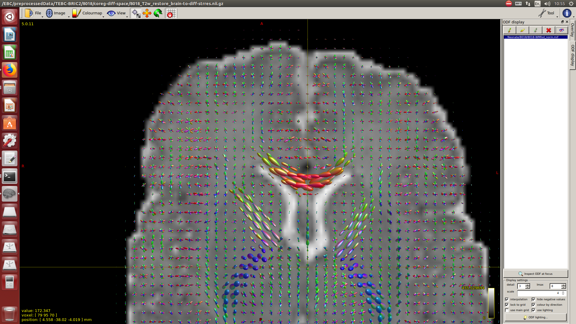
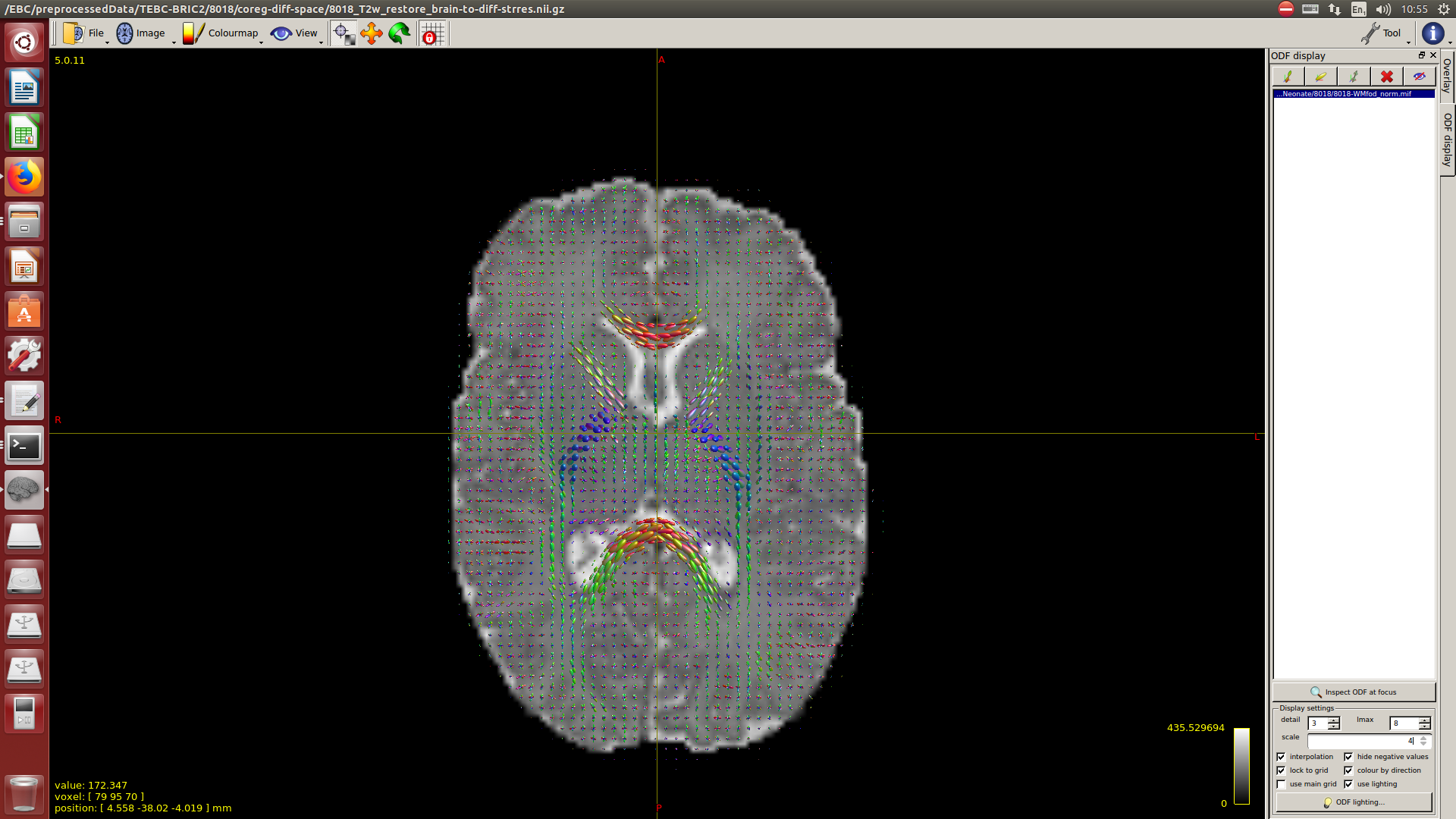
And then dwi2response with dhollander algorithm and -fa 0.1, dwi2fod using only the average WM and CSF response functions (note there is an improved version of the algorithm, also able to correctly detect 3-tissue reponse functions in neonates) and mtnormalise.

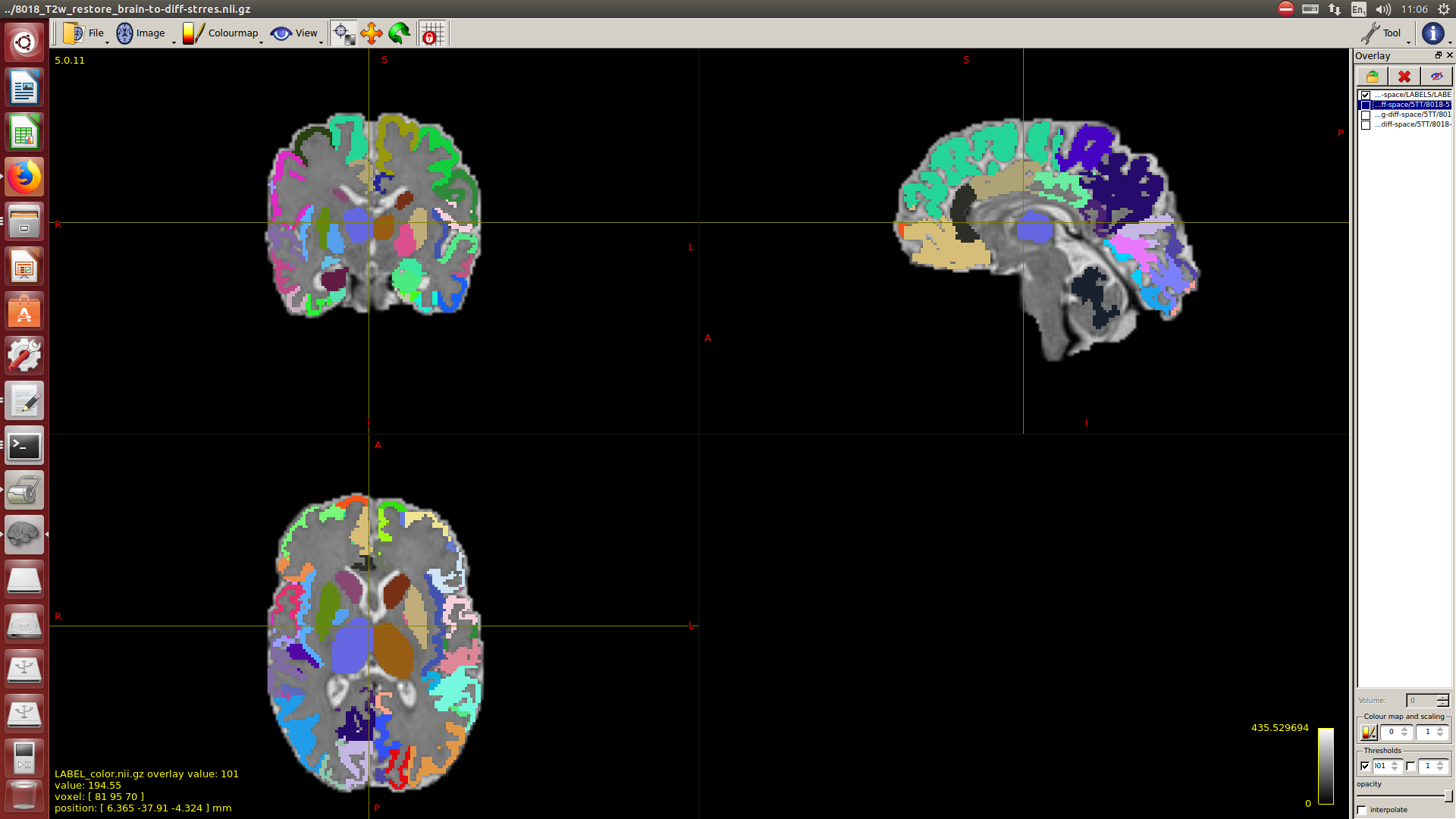
Then a combination of the DrawEM algorithm and M-CRIB atlas for parcellation and obtaining the 5TT file necessary for ACT.

Here you can see some of the results in case you are interested:

I hope this helps,

Best regards,

Manuel