Dear MRtrix3 experts,
I am fairly new to using MRtrix3, so please excuse a fairly basic technical question:
I visualized the response function estimation of my dti data (b=1500, 2x64 directions) with the values 303.4892197 -153.3113817 47.84516512 -10.20100441 1.233455441.
It looks flat and broadest in the axial plane (as I guess it is supposed to).
My question is:
Are there “normal values” (depending on gradient strength / directions) to check the quality of my (individual) DTI data?
Would that even be sensible / intended?
Maybe I did not understand the concept of the response function correctly, so any insights would be appreciated.
Hi,
So there are certain expectations regarding how the response function ‘should’ look; for instance:
- The magnitude of the first term should be approximately the mean DWI image intensity in the white matter.
- From left to right, the values generally decrease by a factor of ~ 3-5, and switch sign between alternate values.
- Ideally, the magnitude should decrease monotonically from the X-Y plane toward the Z axis, though it’s not uncommon for there to be a little ‘bulb’ along the Z axis.
Regarding the appearance itself, the example that comes to mind is Donald’s paper, where one of the figures shows estimated responses from b=1000-5000 - but as angular plots rather than surfaces.
We’ve toyed with the idea of providing pre-defined response functions for particular b-values, as we expect the shape to be dependent on the b-value only; though receiver coil gain and SNR may also play a part.
Probably the more appropriate test to do for the sake of quality control is to check the locations of the voxels used to estimate the response function (-voxels option in the dwi2response script). These should make sense anatomically as single-fibre regions, and should appear to contain a single fibre following application of CSD.
Rob
Hi @TCsquared,
I’ve cross checked the SH coefficients of your response function with those from Donald’s paper (one eye closed, and engineering-wise interpolating a bit between the b=1000 and b=2000 responses in there), and the values definitely sit in the right ballpark!
The shape that you describe is indeed the correct one: the response should look like a softly blown up disk. I’d say, give it a shot and throw your data and response function at dwi2fod: if the FODs look sensible and not too corrupted by false spurious peaks, you should be good.
Cheers,
Thijs
Dear Rob and Thijs,
Thank you both for your helpful advice! Donald’s paper indeed helped clarifying my questions too!
I a designing a pipeline for data processing and will include a step just to visually check the response function.
Again, thank you for your advice!
Bastian
Hi Rob and Thijs,
Using the currently available dhollander algorithm on a single shell data (b0 + b=700) I get the following response_wm.txt:
1459.49618465773 0 0 0 0 0
774.990944178362 -204.206544862093 27.5709543467232 -3.01704665781447 -0.0572831028918161 0.303581684085567
Which the second row looks like this:
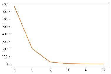
The drop from first to the second term is about 3 times but afterward is more than 5 times and the last element has a bigger magnitude compared to the one before it.
Is this completely wrong?
Nope, it’s perfectly fine. Take a look at it using shview to confirm: I’ve checked, and it looks good.
Is this completely wrong?
Generally what you’re looking for in a response function is:
These data fail to follow the expected shape beyond l=6, which is unsurprising given the lower b-value. What I’ve not had access to data to test is whether or not it is detrimental to retain those higher degree coefficients for spherical deconvolution nevertheless, or whether it would actually be preferable to truncate the response function; feel free to muck around with this.
In a lot of scenarios, that’s what would typically come out, but I wouldn’t personally call it “what you’re generally looking for” in all cases. In low b-value data such as @zeydabadi’s, I’ve observed exactly what Mahmoud obtained here as well. I’m not surprised here; the response furthermore does show the expected shape in the amplitude domain. Including these coefficients in CSD, in my experience, is not detrimental. Due to the low b-value and thus low angular frequencies dominating anyway, the difference is naturally so small that you can barely observe it in the outcome. That said, theoretically, it’s in your favour to not truncate, to avoid other (theoretical) artifacts. That said again, I should probably mostly stress that in practice, you won’t notice any substantial difference though.
Long story short: Mahmoud, I’ve actually inspected the response function you provided here, there’s no reason to worry about it. Note that, by default in any CSD algorithm now, the very last coefficient there won’t even be used (see CSD on standard DWI data - #5 by ThijsDhollander and No lmax=8 cap in dwi2fod msmt_csd · Issue #899 · MRtrix3/mrtrix3 · GitHub). Further do note that, the lmax=10 coefficient, even though seemingly discarded later on given all defaults, does serve a role in response function estimation (see ZSH & amp2response by Lestropie · Pull Request #786 · MRtrix3/mrtrix3 · GitHub and Integrating amp2response in dwi2response scripts by thijsdhollander · Pull Request #862 · MRtrix3/mrtrix3 · GitHub where this was implemented and brought about some other stuff). Omitting lmax=10 at that (response estimation) step is not the same as truncating it down the track: in the response estimation, it can avoid the monotonicity and other constraints to otherwise potentially bias the estimation of (some of) the response ZSH coefficients.
For intuition, you should mainly check your response functions in the amplitude domain, using shview. use the left and right arrow keys on your keyboard to switch between b-values, e.g., to switch from the b=0 to the b=700 part of the response. Use the Escape key to rescale the visualisation if due to switching b-values, the visualisation would appear too small (when switching to a higher b-value) or too large (when switching back again to a lower b-value).
