Average response function does not fit for every DWI data

Dear Matrix users,

Our multi-shells DWI data had a large variation of estimated response function, using “dwi2response dhollander”, between subjects. At least one data set dose not like the kernel(s) of the average response function.
See attached for the snapshots of “tissueRGB” maps, one was created by using the average response functions and the other, individual response function.
Here is the numbers of average wm response
7295.03665 0.00000 0.00000 0.00000 0.00000 0.00000
3669.53434 -1352.01670 278.32229 -33.86468 3.77038 -1.35230
2534.50408 -1245.96384 468.61706 -116.92114 17.38030 -2.05282
2040.47597 -1029.02168 500.42672 -180.25738 46.21569 -8.26366

, the individual wm response kernels,
3467.51261664556 0 0 0 0 0
3067.47740044654 -690.651550608833 112.077164167387 -65.9353320070272 -14.4002764641077 33.4209532489987
2146.20727958034 -696.126351725529 185.491290900128 -29.1255165825243 9.93399894120639 -6.45458943873387
1918.89149067549 -719.806161009428 306.894104139019 -108.458678932664 32.7108502845384 -24.5046883566933

Thanks.

Ping

Hi Ping,

I hope you’re doing well!

There’s a few things that might be going on; though it’s hard to figure out only from the information provided. First and foremost, seeing variation in estimated response functions across datasets can be completely normal if it’s about the general (absolute) scaling of the response functions. So directly looking at those numbers themselves doesn’t tell you much about the variation in shape or contrast between those numbers. It’s the latter that is relevant.

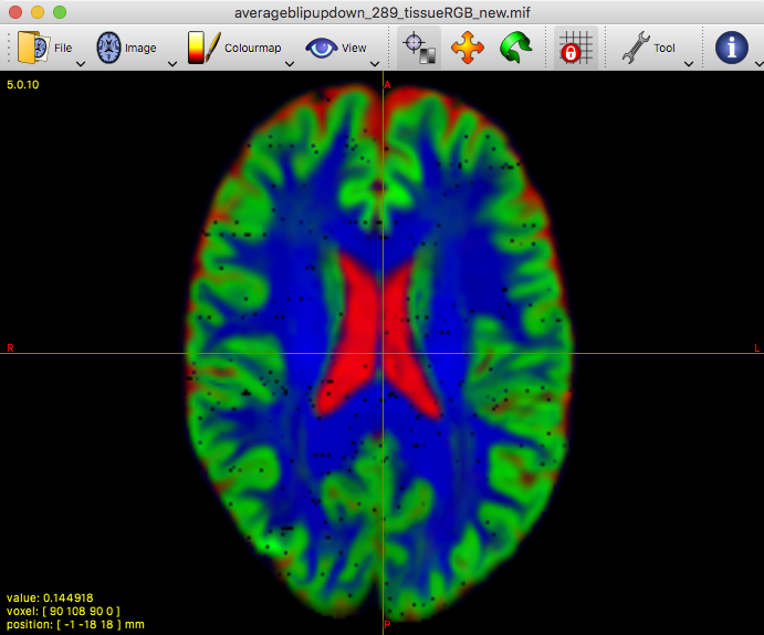
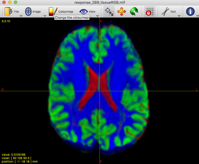
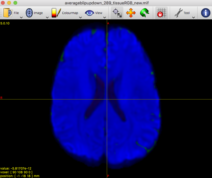
That said, I’ve taken a look at your average WM response function: that looks completely fine actually. Taking into account the successful 3-tissue result you’re showing in the first screenshot using that average response function, I reckon the average WM response function as well as the average GM and CSF response functions are in good condition. Note the latter 2 (GM and CSF) response functions are equally important as the WM response function; they all work together in the modelling result you show in the end!

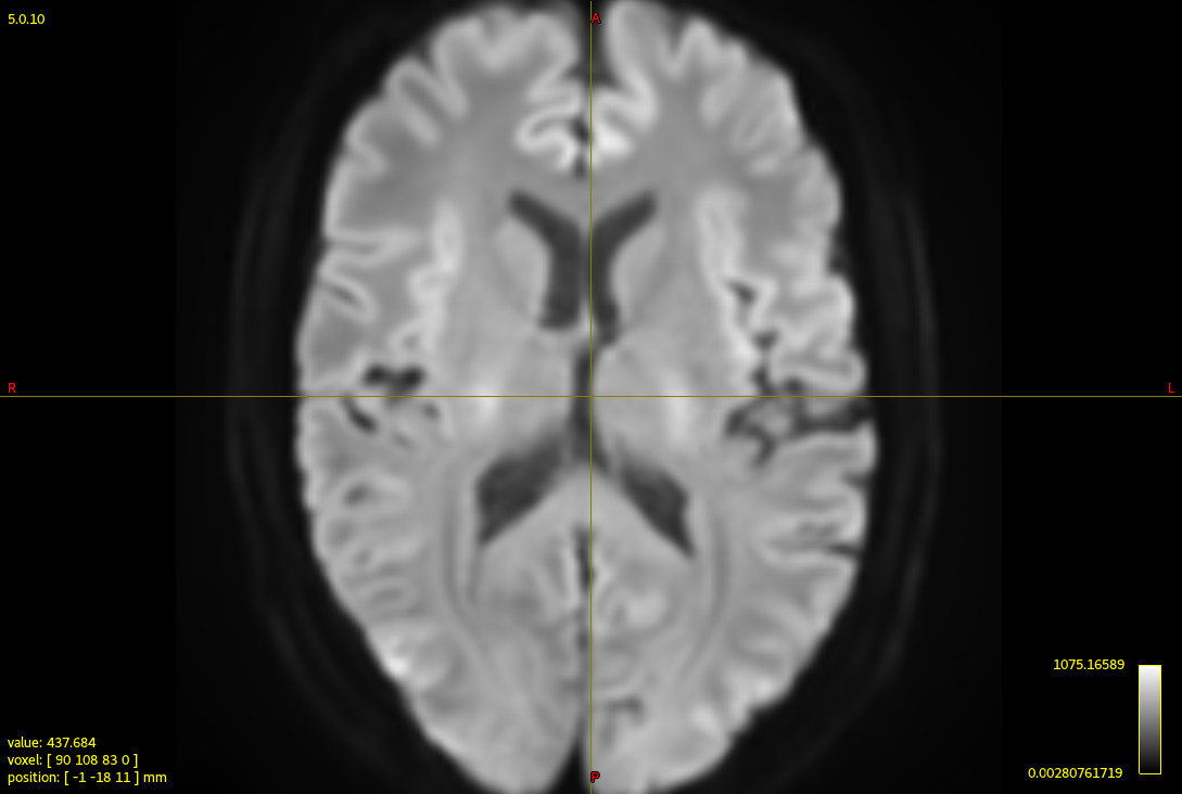
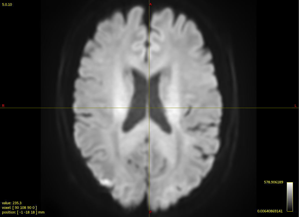
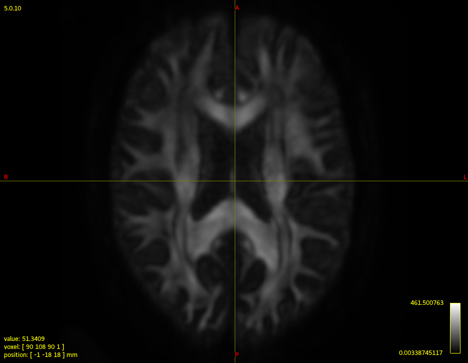
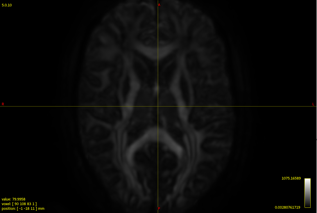
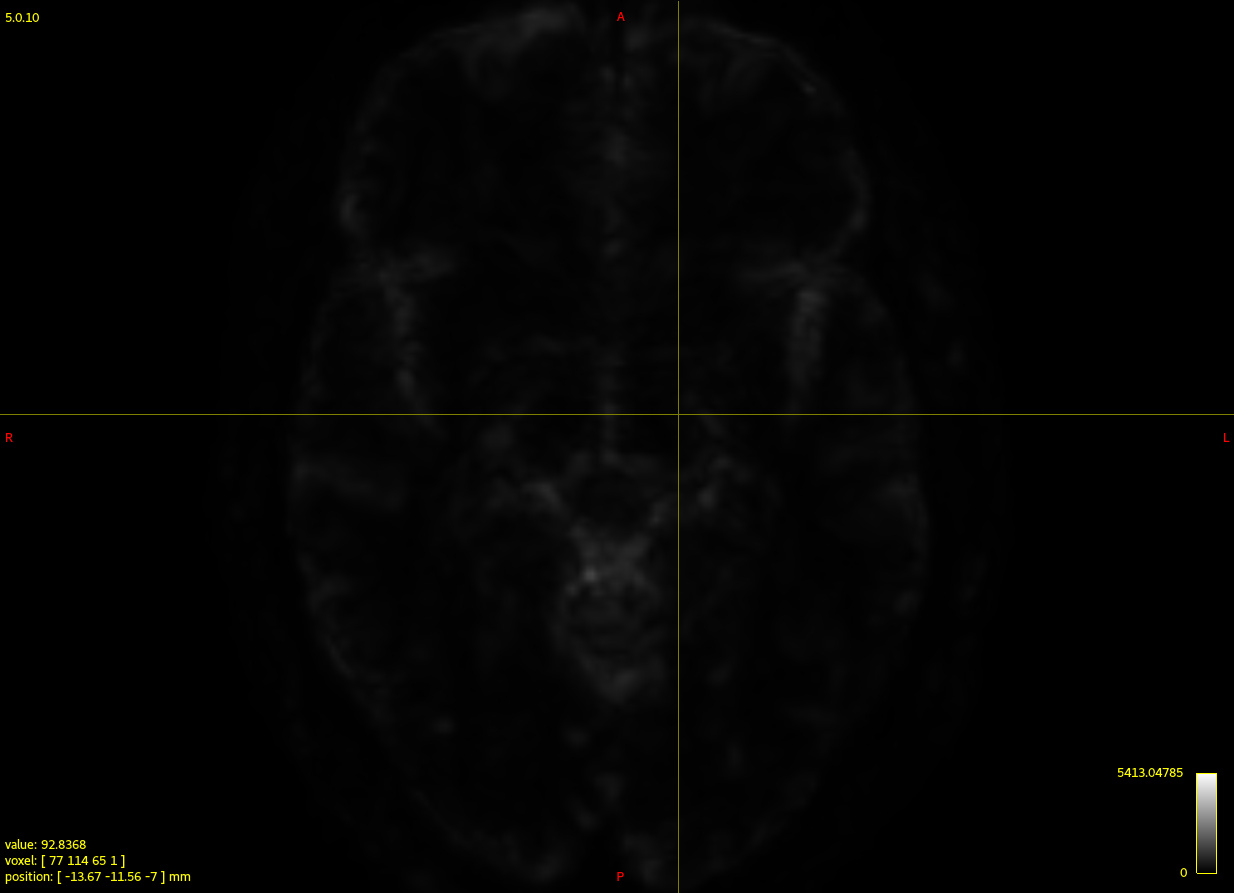
Clearly the second result you show isn’t desirable. Also, that particular individual WM response you show (not the group one) does look different in shape and contrast compared to the average one. Also, even in and of itself it doesn’t look quite right, given certain properties you’d expect for a WM response function.

First things first: aside from your worries about the one individual response function, given your results with the average response functions, I would currently not worry and proceed to use the average WM, GM and CSF response functions without worries across all datasets. The one tweak you could do is to not include the one individual response function you showed into the calculation of the average response function. However, if you’ve got enough subjects, I reckon one individual one will have had very little to almost no impact on the average. So again, I don’t think there’s a great concern of worry per se. Happily continue your analyses in the meantime, I’d say. The other variation, as I mentioned above, is likely only in absolute scale of the response functions. The evidence there is that your average WM response function looks quite good; in a way you’d not expect if the shapes varied too much. So once more, all good I think.

On the side, it’d be nice to figure out what went wrong with the response function estimation of that one individual in particular. Maybe something strange is going on with the dataset itself that you might want to be aware of for example. If that’s the case (e.g. due to some artifact, etc…), there might be reasons to exclude the subject from your study even; so it might be useful to know. Would you be able to share the dataset with me? Feel free to let me know if so, and we can arrange something to make it happen efficiently. In the meantime, it might be handy to mention a few properties about the data: what b-values were used, how many directions, how many b=0 images, etc…? Also, how was the multi-shell acquisition performed: was it all in a single scan, or was it via separate scans for each b-value and did the scans still have to be concatenated in the end? The latter might give rise to some issues that might explain at least some of the things seen in that individual subjects response function.

Cheers,
Thijs

As you’re showing a sensible tissue RGB map generated using the subject-specific response function followed by a nonsensical one for which the average response function was used, assuming other datasets’ average response RGB maps look fine, it seems that this is a data issue for that particular subject, not a response function estimation issue.

I’d say no need to be roped into sharing your data at this point but as Thijs mentions, make sure all DWIs in your study were acquired with the same protocol: TR, TE, and in particular the same diffusion weightings

for dwi in dwis/*.mif; do echo $dwi; mrinfo "$dwi" -shell_bvalues; done

and, as Thijs hinted at, if your individual dMRI data were acquired as a series of separate scans, they can exhibit potentially arbitrary intensity scaling between each other which needs to be corrected for. The script dwicat, part of the development branch, can take care of this if each scan contains at least one b=0 image.

Cheers,
Max

The original post’s wording suggests to me that it is the other way around in terms of screenshots. The quality of both response functions would be consistent with that, as would be the MSMT-CSD result even in that case. If that’s not the case, this should be clarified first.

?

Ok, the file names in the title bars of the screenshot suggests they might be swapped though. Ping, can you clarify which is which?

Hi Thijs, Max,

Thank you for the prompt replies and detailed information.

Sorry for the confusion. Yeah, the screenshots were swapped, the “averageblipupdown_289_tissueRGB_new.mif” was recon using average response function.

Our DWI data were acquired with 3-shell (bvals: 1000,2000, 3000; 90 directions for each shell ) and several b0 (19 volumes) blip-up and blip-down using GE multi-band sequence. Both sets of DWI (blip-up and -down) were concatenated from 2 seperate acquisitions due to the limit of maximal number of volumes =150. DWI data were preprocessed using the TORTOISE package, including noise reduction, eddy current correction, warping to T2W structural image) and combined to one set of DWI followed by bias correction (using MRtrix3 dwibiascorrect).

Let me know if you would like to take a look of data.

I will check if there is scaling issue of DWI; but probably not because other DWIs seemed fine except this particular data set (for now).

Now I have other issues with FOD recon, some of the results have Swiss chease-like brains (voids) (see attached). I was using different computer systems (MACOS, Centos) for processing and suspecting FOD estimation algorithms might fail in some of systems, but I was not able to figure out what caused this. Any insights in debugging? Thank you.

Ping

Here is example of chease-like brain

Hi Ping,

Thanks for clarifying. In that case, some of my explanation above doesn’t hold, as I was reasoning on the other ordering of the screenshots. No worries about that! Just a confusion; it happens. :slightly_smiling_face:

It looks like the problem is separate from response function estimation, and dwi2response dhollander has no issues here. :+1: 
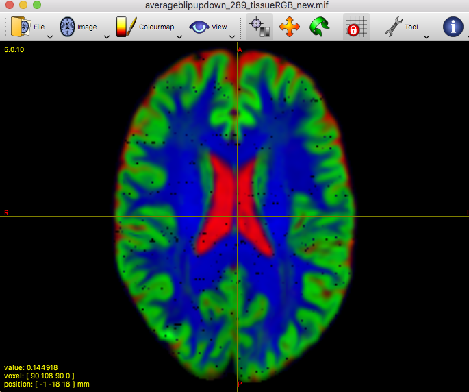
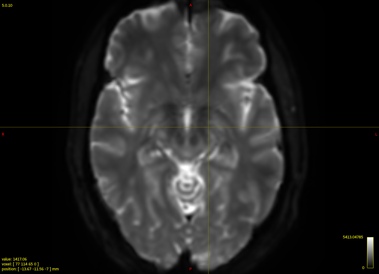
On the contrary, it allowed to reveal that there must be a problem at least with this particular subject’s data earlier on in the pipeline.

It’s important to investigate it, as whatever is the explanation, it might be happening in varying degrees for different subjects in your data, but might only show so extremely for this subject for example (but that might also not be the case; we can’t know for sure). If this happens variably, then the average WM (and other tissues) responses might be off as well, even though they seem to perform well on average. Again, hard to know. The signal decay differs quite a bit between both responses; this is quite telling. The Swiss cheese pattern is another reason of course to go back a few steps in preprocessing and figure out what’s going on.

No need to share data; Max seems quite emboldened to help you out and guide you through debugging remotely. I will kindly take a step back for now while he does so.

Cheers & take care!
Thijs

Hi Ping,

I am not familiar with the TORTOISE package so I don’t know whether it can handle differently scaled DWI data. If not and if your input to the TORTOISE preprocessing consists of two images from separate acquisitions then the preprocessing and the resulting processed data might be affected by data scaling issues due to scanner re-calibration between acquisitions.

I’d suggest you check for each subject that all b=0 volumes have roughly equivalent intensities after preprocessing:
dwiextract dwi_preproc.mif -shell 0 - | mrstats - -output median -mask mask.mif

and if in doubt visually inspect these
dwiextract dwi_preproc.mif -shell 0 - | mrview -

If intensity scales vary across b=0 volumes, use dwicat to normalise the raw DWI data prior to preprocessing (mrconvert -coord allows you to split the concatenated data if needed. Once your data is fixed and preprocessed, you’d need to re-estimate response functions, then average response functions and finally perform MSMT CSD.

Do you get different MSMT results on different systems? To check whether the pepper-noise is already in your preprocessed data have a look at the data by shell, using dwishellmath with arguments mean and std or manually:

for b in `mrinfo dwi_preproc.mif -shell_bval`; do mrcat $(dwiextract dwi_preproc.mif -shell $b - | mrmath - mean - -axis 3) $(dwiextract dwi_preproc.mif -shell $b - | mrmath - std - -axis 3) -axis 3 - | mrview - ; done

Cheers,
Max

Hi Max,
Here is number of median of all mean b0 volumes
1714.43
1692.27
1693.71
1697.18
1697.74
1684.57
1664.22
1704.57
1682.47
1673.43
1661.48
1674.72
1580.79
1632.3
1662.79
1666.44
1661.48
1658.92
1648.9

It seems to me one volume is a bit off, otherwise not too bad.

Attached are the screenshots of mean and std of each b values from one preprocessed data. There is no evidence of pepper-noise.
What puzzles me is that the results from earlier runs seemed fine (see attached “averageblipupdown_289_tissueRGB”, but now is bad (“averageblipupdown_289_tissueRGB_new”). I am not able to reproduce the earlier results.


Thanks.

Ping

Yes, slight drift and possibly one outlier (does that volume look normal?) but otherwise nothing obviously wrong with the median intensity. I’d suggest you run this check on your other data as well just to be on the safe side.
image

To debug this we’ll need more information:

  • Do you get different MSMT CSD results on different systems using the same data and response functions?
  • Was MRtrix3 compiled on the system that produces the problematic images or was it copied from another system? Is it a standalone build? If not done already, could you retry with MRtrix3 compiled from source on that system?
  • Could you provide the config files for both systems?

Cheers,
Max

Currently, the runs on different systems for problematic data all get bad results.
All MRtrix3 were compiled from the source codes, if I recalled it right.

See attached for dwi2fod log files from one of Centos virtual machines and standalone Centos. The MacOS one was similar to those. centos_dwi2fod.js (16.3 KB) centos_standalone.js (16.3 KB)

Thanks.
Ping

re-run using the latest release of MRtrix3 on a MACOS, sill problematic.

dwi2fod_mac.js (9.6 KB)

Hi Max, Thijs,

I’ve copied data to a local machine and re-run dwi2respnose, and the results appear ok.
I think those cheese(pepper)-like artifacts are probably caused by a running-low storage space of our server.
I am running population template creation and other steps for FBA, can a low storage be problematic?
I have more than 400 DWI data sets.

Sorry for the false alarm and thank you for your help.

Ping