Hello,
I’m currently working on a project in which one of the main goals is to compare the tractography algorithms of MRTrix and FSL.
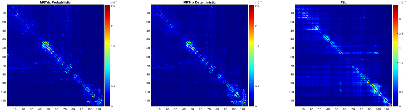
In MRTrix, I performed the tractography initially using SD_Stream (deterministic) and in FSL I used probtrackx (probabilistic). However I found that the resulting connectivity matrix was quite different and I thought the difference could be because of the nature of the algorithms (deterministic vs probabilistic). Having said this, I redid the MRTrix tractography now using the iFOD2 (probabilistic) option in tckgen, and the results were very similar to the ones of the deterministic option which was still quite different from the FSL result. Attached I include an image with the 3 connectivity matrices.
Do you have any clue as to why there can be such a difference between MRTrix and FSL tractographies (especially between both the probabilistic algorithms)?
To be noted that I used the same normalisation of streamlines (normalised by the volume of the ROIs and by the total number of streamlines seeded) and although FSL does not have the option to use the ACT framework (which I used in MRTrix) I included the GM/WM interface as a termination mask. Other things I did in the MRTrix pipeline and not in the FSL pipeIine was performing sift2 and normalising the FOD with mtnormalise.
I hope you can help and thanks for your time,
Ana
Hi Ana,
I’m not sure what’s causing these differences, but it’s at least reassuring to see that the results from both deterministic and probabilistic MRtrix approaches are so similar. This makes sense given they both use the same source of orientation information (some variant of CSD, though I note you don’t mention which one?).
I assume you’re using BEDPOSTX as the source of orientation information in FSL? If so, I’d expect the b-value and SNR to both have potentially quite a large impact on the results, given its Bayesian implementation and the use of Automatic Relevance Determination to figure out the likely number of fibre populations. In high noise or low contrast (low b) situations, there will be little evidence to support high numbers of fibre orientations, and the method will tend to underestimate the number of fibre populations (see e.g. Figs 8 & 9 in the original Neuroimage 2007 paper) – at which point there is no guarantee that the directions estimated will be correct. In contrast, CSD makes no attempt at figuring out the number of populations, and high noise / low contrast situations just lead to noisier results (e.g. more spurious peaks, inaccuracies in the peak orientations). That could account for some of the differences.
I also note that the matrix produced using the FSL pipeline is not symmetric, which is unexpected: this implies that the connectivity (A→B) ≠ connectivity (B→A), which doesn’t sound right (the dMRI signal is antipodally symmetric, there is no information from which to infer asymmetric connectivity values). Maybe there’s a trick I’m missing here – if so, I expect someone will soon correct me…
Just my 2¢…
All the best,
Donald.