Hi MRtrix community,
We are currently performing an exploratory connectivity-based parcellation of the STN from an existing GPe–STN tractogram, as part of a revision of a manuscript.
The aim is to determine whether the connectivity of STN voxels with the GPe naturally supports a discrete clustering structure, and in particular whether the data support 2 or 3 connectivity-based subdivisions.
For each STN voxel, we constructed a connectivity fingerprint describing its connectivity with the GPe voxels. The tractogram itself is already genetated the idea is not to re-run tckgen for this analysis.
The fingerprints are normalized and square-root transformed, and Ward hierarchical clustering is applied directly to these feature vectors:
feats = np.sqrt(fingerprints[connected])
Z = linkage(feats, method="ward")
Thus, Ward operates directly on the square-root-transformed connectivity fingerprints using Euclidean geometry.
The Pearson correlation matrices shown next to the dendrograms are calculated separately and only used for visualization:
corr = np.corrcoef(feats)
order = leaves_list(Z)
corr_reordered = corr[np.ix_(order, order)]
Pearson correlation therefore does not enter the Ward clustering itself.
I have attached the results from our three independent high-resolution ex vivo specimens.
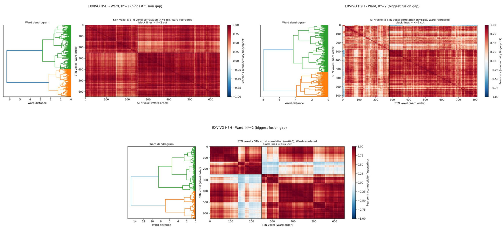
In all three specimens, if we define the “natural K” as the number of clusters corresponding to the largest gap between successive Ward fusion heights, the result is K=2*.
We then also cut exactly the same dendrograms at K=3, because three subdivisions are of particular biological interest in our study.
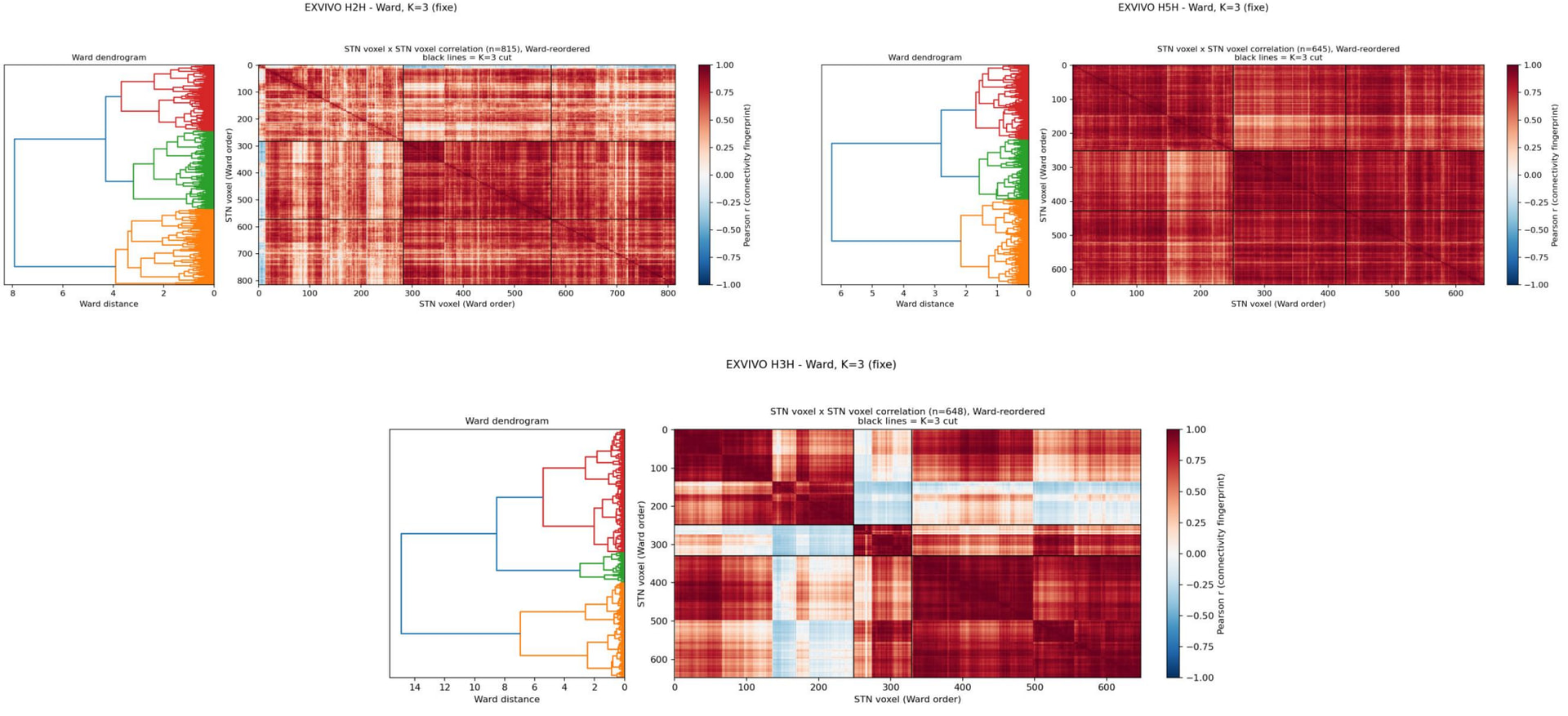
What I find interesting is that K=3 does not seem to produce three equivalent major branches. Instead, visually, the main K=2 division appears to remain and one of these two branches is subsequently subdivided:
A / B → A / (B1 + B2)
rather than:
A / B / C
The corresponding Ward-reordered fingerprint correlation matrices also seem quite different between specimens: H3H shows particularly strong block structure and even negative correlations between some groups, whereas H5H appears much more globally correlated, with H2H somewhere in between.
I would therefore be very interested in your interpretation of these plots.
Specifically:
1. Is it reasonable to interpret the large final Ward fusion gap observed in all three specimens as evidence that the strongest level of organization is a two-cluster division?
2. When cutting the same hierarchical tree at K=3, is the pattern we observe reasonably described as a hierarchical subdivision of one of the two principal groups rather than evidence for three equally distinct clusters?
3. How much weight would you give to the block structure of the Ward-reordered Pearson correlation matrices when judging whether the clusters are meaningful?
For example, H3H seems to show much stronger differentiation between connectivity fingerprints than H5H, despite both having K*=2.
4. Is the “largest successive fusion-height gap” an appropriate way to describe the natural K for Ward clustering in this context, or should this only be considered descriptive and complemented by other cluster-validity/stability measures?
5. Finally, can Ward fusion distances be meaningfully compared between specimens, or should their absolute magnitude only be interpreted within each dataset?
Our current interpretation would be that these results show a reproducible dominant bipartite organization, with additional hierarchical structure that can generate a K=3 subdivision, rather than three equally well-separated connectivity clusters.
However, we would really appreciate opinions from people more experienced with connectivity-based parcellation and hierarchical clustering before making this interpretation in the manuscript.
Many thanks for your help.