Hi Roey,
I suggest taking the dimensionality analysis offered in the OHBM Aperture 2022 article, and the thought experiment of globally scaling brain size as utilised in this FBA work, and mashing the two together.
Imagine taking an FOD image and corresponding tractogram, and scaling both along all three spatial axes by a factor of 2. The number of streamlines in the tractogram remains fixed (similarly how one may generate the same number of streamlines in each study participant regardless of brain size). We assume also that the tractogram contains no biases for SIFT2 to correct. Streamline lengths will increase by a factor of 2, while the number of WM voxels will increase by a factor of 8.
We now have to split the thought experiment in two, depending on what we infer to have happened to the underlying tissue and hence the FODs:
-
The set of underlying fibres were to be completely unchanged in both count and caliber.
The intra-axonal volume fractions, and hence the sizes of the FODs and correspondingly fixel-wise FDs, would scale by around 1/4.
The value of mu would be unchanged. The sum of fibre densities would increase by 2 (8 times as many fixels, 1/4 the FD per fixel), and the sum of streamlines density increased by 2.
Measurement of FBC would yield an unchanged result.
This is entirely consistent with my premise of this first scenario:
The set of underlying fibres were to be completely unchanged in both count and caliber.
-
The “packing density” / intra-axonal fractions were to be unchanged.
The additional space afforded by the expansion is occupied by additional axons / expansion of axon caliber (ignoring here the influence of loss of restriction in very large axons on the DWI signal).
Presume that this occupation of the bonus space magically results in 4 times the intra-axonal cross-sectional area, since that is what leads to no change in intra-axonal volume fractions, hence the FODs being of the same size as that of the original brain, with correspondingly equivalent fixel FDs.
The value of mu would go up by a factor of 4. The sum of FDs would go up by a factor of 8, due to 8 times more fixels each with unchanged underlying FD values, and as stated the sum of streamlines lengths goes up by a factor of 2.
This will result in a reported increase in FBC by a factor of 4.
If you were to repeat this experiment across a wide range of brain sizes, then you would find a linear relationship between mu and FBC.
If the scale factor applied to each of the three spatial axes were A, then you would expect FBC to scale as A2/3. For bonus points, consider the relationship between this and the FC metric in FBA.
The argument I made in Aperture 2022 is that this is the correct answer.
In a brain that is 8 times larger, you can fit in 4 times the intra-axonal cross-sectional area. If you utilise the exact same parcellation, then each endpoint-to-endpoint connection has the prospect of inheriting that 4x increase. This is a genuine difference in these two brains in “the information-carrying capacity of those connections”, at least as long as one accepts the premise that “more axons == more connectivity” and “larger axons == more connectivity” and a bit of gesticulation.
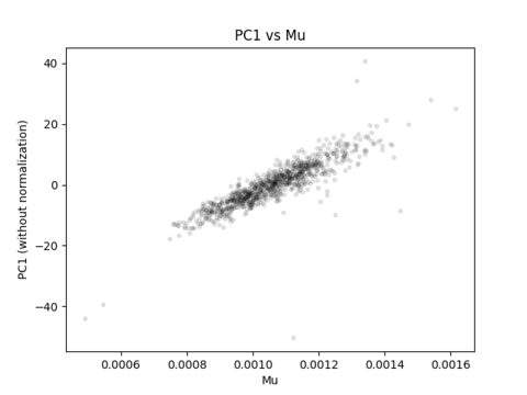
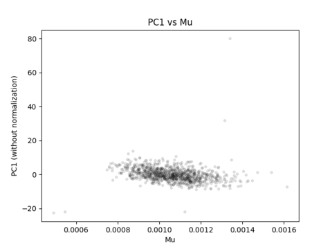
What your correlation between PC1 and mu is actually capturing is the fact that you have brains of different sizes, but are generating the same number of streamlines per individual.
Imagine for instance that you were to be able to terminate tractogram generation at the point in time at which the value of mu reaches some value (similarly to how in tcksift you can terminate filtering upon reaching a certain value). You would then most certainly not see any correlation of a principal component with mu, because the inter-individual variance in mu would be at the precision of streamline count quantisation.
mu is neither a dimensionless latent variable, nor is it intended to squash all correlations between all variables. Its appropriate use is intended to provide quantities that scale suitably with the underlying connection density. Sometimes there are things other than “the esoteric behaviour of probabilistic tractography” that streamlines-based connectivity will scale with. That doesn’t necessarily mean that those are unwanted correlations. Eg. Maybe a bundle end region is bigger because it requires more connectivity, and so explicitly dividing connectivity estimates by end region cancels the effect of interest.
It is certainly an option to do an explicit “normalisation” of sorts of connectome values, whether by the total density in the connectome or by the total connectivity in the tractogram (arguably better IMO). Another point I tried to make in Aperture 2022 is that this is not just a matter of “hey, here’s an experimental factor, let’s regress against it”. It’s a fundamental change in your quantitative parameter. You are no longer quantifying “the information-carrying capacity” of the bundle, but rather “the fraction of whole-brain information-carrying capacity that belongs to this bundle”. If that suits an individual application, then so be it; but it should be done with both intention and understanding.
In retrospect, perhaps in this submission I should have explicitly included “fraction of streamlines” as a connectivity metric to debunk…
Regards
Rob