Ex-vivo mouse brain FBA

[araikes]

Greetings all,

I’m hoping you can help me out here. I’m working on a dataset of ex-vivo mouse brains. We collected 0.2mm isotropic imaging with 3 shells (b1000, 2000, 3000 +b0) and 64 directions per shell. Initial preprocessing (including reorientation of the images and eddy correction) was done using TORTOISE.

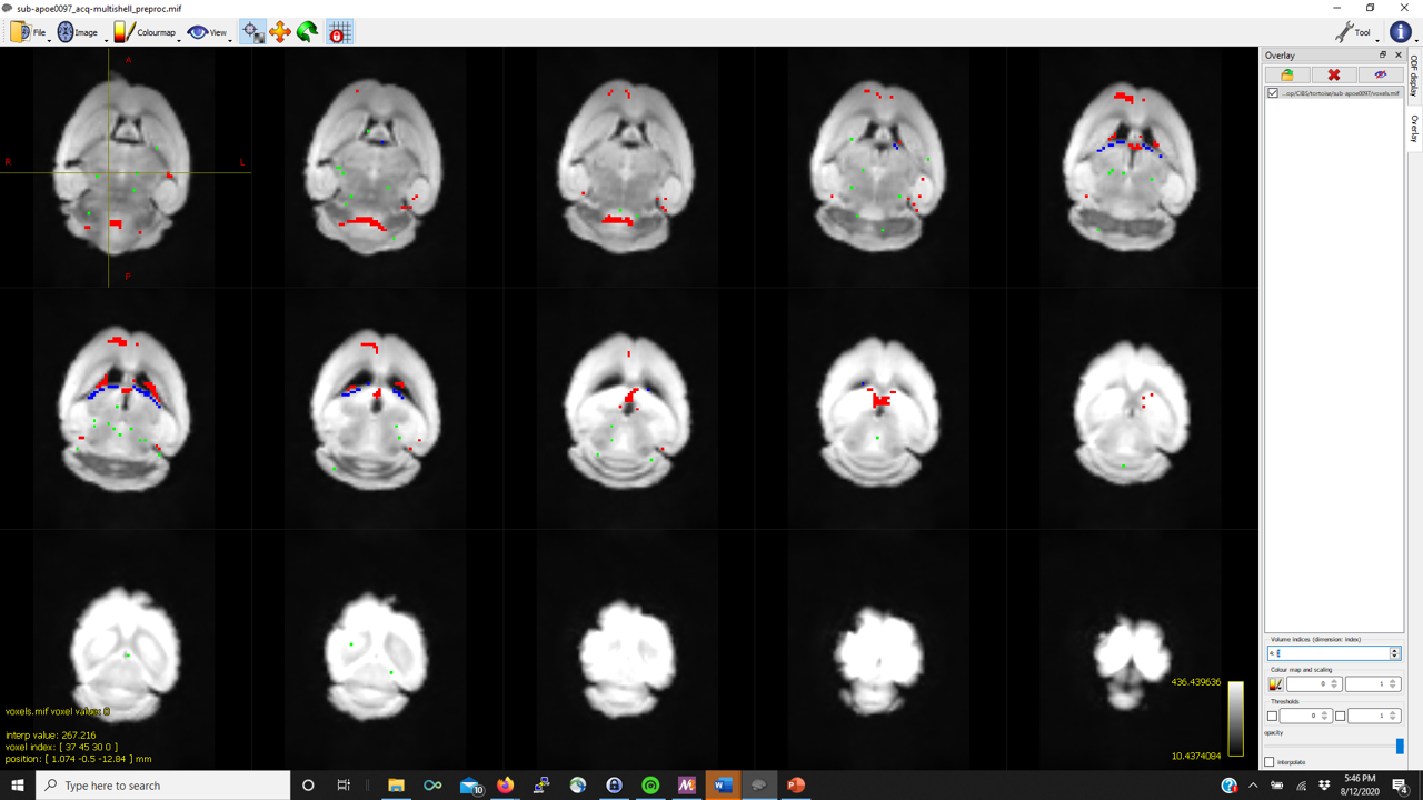
I’m trying to run the FBA pipeline described in the documentation. dwi2response dhollander produces reasonable WM FODs but struggles to detect good representative CSF voxels. As such, in several of the mice, mtnormalise has a negative tissue balance such as

 [WARNING] For input "sub-apoe0097" (returncode = 1):
          mtnormalise: [WARNING] existing output files will be overwritten
          mtnormalise: performing log-domain intensity normalisation... []
          mtnormalise: [ERROR] Non-positive tissue balance factor was computed. Balance factors:   4.3531205638674342    3.559592222662189 -0.41592815237490682

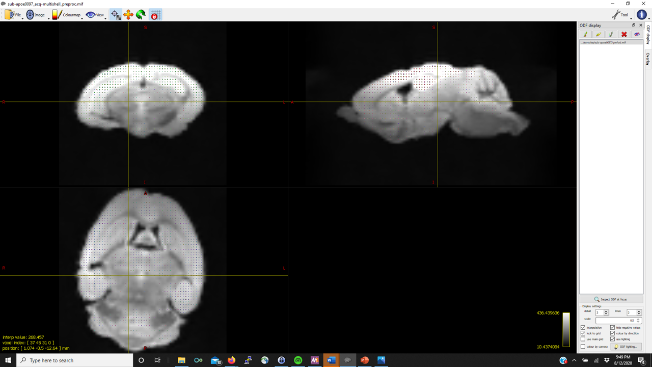
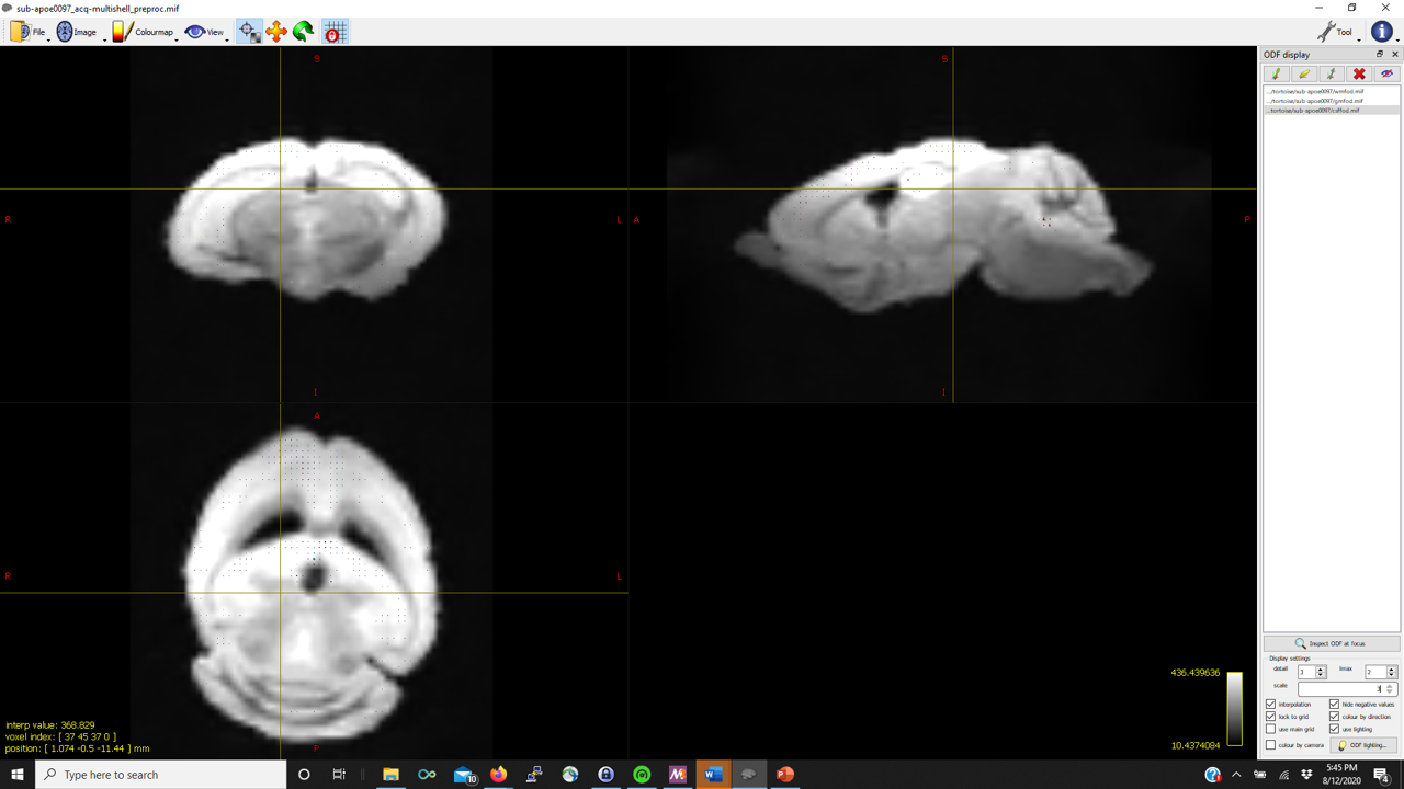
However, the gray matter FODs are fairly reasonable and well-placed (in contrast to other posts on the community) in almost all of the mice.

I know there was a suggestion in a post somewhere (not finding it right now) to use a 2 tissue WM-CSF mtnormalise but I’m wondering if a WM-GM mtnormalise would be a valid strategy.

Thanks in advance (pictures below for WM, GM, CSF FODs and the voxel image from dwi2response from a representative mouse that fails mtnormalise)

[ThijsDhollander]

Hey @araikes,

Long time no see; hope you’re doing well!

@araikes

I’m hoping you can help me out here. I’m working on a dataset of ex-vivo mouse brains. We collected 0.2mm isotropic imaging with 3 shells (b1000, 2000, 3000 +b0) and 64 directions per shell. Initial preprocessing (including reorientation of the images and eddy correction) was done using TORTOISE.

For ex-vivo data, we find that using a very high b-value is sometimes crucial to get angular contrast and proper sensitivity to intra-axonal signal. This is typically a factor higher than for in-vivo data. In your case, in this context, the b-values aren’t very high. For such ex-vivo data, mouse specifically, I’ve recently seen benefit using just the highest b-value you have, and b=0, with SS3T-CSD to get a better resolved result, i.e. more cleanly defined FODs even in presence of the massive amounts of GM partial volume in the mouse cortex. Using just b=3000 and b=0 can help dwi2response dhollander for the same reasons in this scenario.

@araikes

dwi2response dhollander produces reasonable WM FODs but struggles to detect good representative CSF voxels.

Yes, this problem will exist regardless of my above advice. This is because of how little fluid there is in the (relatively) tiny mouse ventricles. Since this is ex-vivo, I suppose the brains have been prepared and are suspended in more fluid? In that case, a somewhat funny pragmatic solution is to dilate your brain mask several times, so the “brain” mask includes more fluid surrounding the ex-vivo brain. This will help dwi2response dhollander in getting sufficient CSF samples, but also restore the WM-GM-CSF balance to something more reasonable for that purpose. We’ve seen this work very well in practice then.

@araikes

As such, in several of the mice, mtnormalise has a negative tissue balance such as

Yes, at that point it was already messed up from the start. Your CSF response was indeed not a proper one, resulting in a problematic CSF-like image, resulting in this problem with mtnormalise. It’s not surprising, but you need to go back to the origin of the problem (response function definition) to fix it.

@araikes

However, the gray matter FODs are fairly reasonable and well-placed (in contrast to other posts on the community) in almost all of the mice.

I know there was a suggestion in a post somewhere (not finding it right now) to use a 2 tissue WM-CSF mtnormalise but I’m wondering if a WM-GM mtnormalise would be a valid strategy.

Good to hear the GM response is then reasonable. WM-CSF won’t immediately help you here since the CSF response itself is the problem. And it would be a bit of a waste, since you’re got a good GM response. However, WM-GM doesn’t fit fluid at all, especially the lower b-values, e.g. b=0 in extremis. Using WM-GM modelling would result in “hyper-GM” in CSF areas due to this. Even though the ventricles are small, this would also affect any occurrences of free water and severely bias the fit there. So your best bet is to find a better CSF response. Either use the strategy above (if there is effectively fluid in the background) or as a last resort, use dwi2response manual specifically for the CSF response (providing it with a mask where you manually segmented a few CSF voxels, just a hand-full is enough for this purpose). Using the latter strategy, continue using the WM and GM responses from dwi2response dhollander but replace the CSF one by the manually obtained CSF response.

Cheers & take care,
Thijs

[araikes]

Hi @ThijsDhollander,

Thanks for getting back to me. I’ll definitely give your suggestions a shot, starting with dilating the masks a bit. To clarify, if I dilate the masks, I should use that only for the tissue responses but then still use a tight mask for mtnormalise, correct?

[ThijsDhollander]

@araikes

To clarify, if I dilate the masks, I should use that only for the tissue responses but then still use a tight mask for mtnormalise , correct?

Yes & no in a way: if the mask doesn’t extend beyond regions with genuine fluid, i.e. reflecting the eventual CSF response, then the 3-tissue CSD fit should also show CSF-like signal in the corresponding region. By virtue of that, the region will be entirely compatible with the mtnormalise assumptions. But since you’re likely not interested in studying that area (beyond just extracting a response from it), there’s no need to even include it in the mask for 3-tissue CSD or any other step. So to keep it simple, yes, you can regard this just as a trick for getting responses and only use it in that context.

This is interesting though: in e.g. human data with strong atrophy or a surgical resection, which creates a larger “non-parenchyma” region filled with fluid, it actually helps to keep this within the mask for all processing, including mtnormalise; it’s in those cases even beneficial in helping correct bias fields more robustly.

Finally, you at least want some CSF-like region in your mask for mtnormalise when doing a 3-tissue fit, otherwise you’ll get other problems. But for that purpose, you should typically be ok with just the ventricles, even as small as they are (relatively) for the mouse brain.

So in conclusion, you should be good with just using your normal masks for everything; and try the dilation trick for dwi2response purposes. Check the -voxels output to see if it helped. If not, finally resort for these data would be dwi2response manual, but only for the CSF response.

[rsmith]

Adam,

If you look closely at the coronal projection with the white matter FODs, you’ll see that your diffusion gradient orientations are not being interpreted correctly. Best to rectify before blowing too many CPU cycles on subsequent processing

Rob

[araikes]

Hi @rsmith and @ThijsDhollander

First and foremost, @rsmith, any recommendation for checking the gradients? These were converted from the Bruker format and denoised/degibbsed/eddy corrected using TORTOISE. The only other step taken was to reorient the image using TORTOISE to LPS but this process also flips the b-table.

Second, I think overall this might be part and parcel of a larger issue. The brains were initially preserved in a fixative (PBS) before being transferred to Fluorinert for imaging. In some mice, the PBS drained from the ventricles but not some of the smaller areas and so the CSF response is being grabbed from residual PBS and not the Fluorinert. For other brains, the PBS didn’t completely drain from the ventricles, so I get a different response in the ventricles than from outside the brain even for those animals. Thus, I have inconsistent response functions across animals for the CSF because of the relative presence/absence of PBS in small and larger areas. It also means I can’t use voxels from the ventricles alone to estimate the response function since this will be inconsistent depending on whether the PBS drained out or not.

For this reason, I’m testing out the SS3T FBA approach using the b0 and b3000 shell. Image of the wmfod for the same mouse using this approach.

[araikes]

@rsmith

Follow-up: Here’s the results from dwigradcheck. I just don’t know what it means.

Mean length     Axis flipped    Axis permutations    Axis basis
 9.34            2                (0, 1, 2)           image
 9.29            2                (0, 1, 2)           scanner
 5.98         none                (1, 0, 2)           scanner
 5.92            2                (1, 0, 2)           image
 5.70         none                (0, 1, 2)           scanner
 5.70         none                (0, 1, 2)           image
 5.67            0                (2, 1, 0)           scanner
 5.66            0                (2, 1, 0)           image
 5.60         none                (1, 0, 2)           image
 5.58            2                (1, 0, 2)           scanner
 5.42            1                (2, 1, 0)           image
 5.41            1                (0, 1, 2)           image
 5.39            1                (2, 1, 0)           scanner
 5.38            2                (2, 1, 0)           scanner
 5.35            2                (2, 1, 0)           image
 5.31         none                (1, 2, 0)           scanner
 5.30            1                (0, 1, 2)           scanner
 5.29            0                (1, 2, 0)           image
 5.25         none                (2, 1, 0)           image
 5.18            1                (1, 0, 2)           scanner
 5.16         none                (2, 1, 0)           scanner
 5.16            2                (1, 2, 0)           scanner
 5.13            0                (1, 0, 2)           image
 5.12            1                (1, 2, 0)           image
 5.09            1                (1, 2, 0)           scanner
 5.07            2                (1, 2, 0)           image
 4.90            0                (1, 0, 2)           scanner
 4.90            0                (1, 2, 0)           scanner
 4.89            1                (1, 0, 2)           image
 4.86         none                (1, 2, 0)           image
 4.64            0                (0, 1, 2)           scanner
 4.63            0                (0, 1, 2)           image
 4.61         none                (0, 2, 1)           scanner
 4.58            0                (0, 2, 1)           image
 4.49            1                (0, 2, 1)           image
 4.47            2                (0, 2, 1)           scanner
 4.31            2                (2, 0, 1)           scanner
 4.26         none                (2, 0, 1)           image
 4.16            1                (0, 2, 1)           scanner
 4.10            0                (2, 0, 1)           scanner
 4.08            2                (0, 2, 1)           image
 4.08            1                (2, 0, 1)           image
 4.00         none                (2, 0, 1)           scanner
 3.95            1                (2, 0, 1)           scanner
 3.95            0                (2, 0, 1)           image
 3.94            2                (2, 0, 1)           image
 3.87         none                (0, 2, 1)           image
 3.86            0                (0, 2, 1)           scanner

[rsmith]

That means that with a pretty high degree of certainty, you need to take your diffusion gradient table and multiply the Z-component of every vector by -1.

Alternatively, you could re-run dwigradcheck with one of the -export_grad_* options, and then use mrconvert to import the recommended modified gradient table back into the image header.