Hi Rob!
Thanks a lot for answering my questions! It will be of great help for my analysis 
I will get in touch if there are further issues 
Hi Rob!
Thanks a lot for answering my questions! It will be of great help for my analysis
I will get in touch if there are further issues
Hello again 
I’m trying to run FBA with data acquired at 2 different sites (different scanners, sequence).
I set the design matrix as
0 1 0
1 0 1
with the 0 in the 3rd column representing data from the 1st center & 1 in the 3rd column representing data from the 2nd center.
Similarly, I set the contrast matrix with an additional 0 as 1 -1 0
Is this the right setup 
Moreover, the pathology is more severe in one of the data-sets as compared to the other.
How can I incorporate this info in my design and contrast matrix 
Thanks,
Karthik
Is this the right setup
If you had provided more rows, then I believe that your setup would be correct. However the very limited matrix that you provide there would lead to severe problems due to under-determinedness; I honestly don’t know how the current master code would react, but I recently observed my development branch code providing t-values of ±1e9 in a similar circumstance, which leads to essentially a stalled command. But if you have more than two subjects, then what you’re describing is correct.
Moreover, the pathology is more severe in one of the data-sets as compared to the other … How can I incorporate this info in my design and contrast matrix
This kind of question really gets to the fundamentals of design & contrast matrix construction. The answer to this question is: What is your hypothesis?
I’m first assuming that you have both controls and patients scanned at both centres. If this is not the case, then there’s no mathematical way of disentangling the effect of variation in pathology severity between sites from the effect of scan site.
From there, how to proceed depends on which of these two cases has caused you to raise the question:
You have some continuous measure of pathology severity, and have noticed that the mean differs in the patient groups between the two sites. How to deal with this depends on whether or not that continuous measure of severity can also be computed for the control group.
The patients that were scanned at one site are subjectively / clinically more severe than the patients scanned at the other site, but this is not quantified. If this is the case, then one would expect the magnitude of the difference between patients and controls to differ between the two sites. This should also be possible to deal with. Though going back to the point about the hypothesis, that question extends to whether this is an effect that you expect to observe in your data and hence with to include in your model in order to provide the best possible fit to the data, or whether you actually want to test whether this effect is non-zero.
There’s a number of possibilities here, and I’m trying to avoid writing a comprehensive GLM instruction manual ![]()
Rob
Thanks for the detailed reply.
Actually, I do have more no. of rows in the actual experiment I just wanted to check if the setup was right!
Yes, both controls and patients were scanned at the 2 centres. I also did an ROI analyis on the FA maps and found a difference in magnitude in the FA values between the centres as expected.
The hypothesis is that the patients should show reduced FBA metrics as compared to controls (also FBA should be more sensitive than DTI in that aspect).
Looking forward to your comments
Karthik
The hypothesis is that the patients should show reduced FBA metrics as compared to controls
Well, in that case your design matrix would only have two columns; either one for each group, or a column of 1’s (global intercept) and then a column with -1 / +1 group assignment. What I’m trying to communicate by asking about your hypothesis is: any nuisance regressors you add into your design matrix in fact form part of your hypothesis.
For instance: Imagine that you simply add a column containing a -1 / +1 corresponding to which site each subject was scanned at. Within the GLM, this will add a factor that attempts to model any global difference in metric values between sites. However this will be applied to all subjects; i.e. the model hypothesizes that values for both patients and controls will be equally larger / smaller at one site than the other. Whereas from your description, it sounds like you are additionally expecting that, independently of the control subjects scanned at each site, the patients scanned at one site are expected to be more severe than those scanned at the other; but they are not so grossly different that you wish to examine patients from the two sites as two separate groups.
What I think you’re looking for (more than happy to be corrected on this), is:
                  GI   Group    Site   Severity
Control, site 1 | +1 |   +1   |  -1  |     0    |
Patient, site 1 | +1 |   -1   |  -1  |    -1    |
Control, site 2 | +1 |   +1   |  +1  |     0    |
Patient, site 2 | +1 |   -1   |  +1  |    +1    |
                ---------------------------------
                  b1     b2      b3       b4
Coefficient b1 encodes the Global Intercept: The predicted value of your quantitative measure of interest after all other predicted sources of variance in your experiment have been factored out.
Coefficient b2 encodes the group (patient / control); a non-zero value here indicates that whether or not a subject is a patient or a control has an effect on the value of the quantitative measure observed in that subject. This is most likely the feature of the experiment that is of interest to you: the null hypothesis is that there is no difference between patients and controls: b2 = 0.
Coefficient b3 encodes the site of the scan. If this factor is non-zero, then whether a particular subject was scanned at site 1 or site 2 has an effect on the quantitative measure observed in that subject - regardless of whether that subject is a patient or a control.
Coefficient b4 encodes the site of scan, but is zero-filled for controls. What this factor therefore represents is the possibility that the severity of the disease (and hence the magnitude of the effect on the quantitative measure relative to controls) may vary between the two sites. For instance, if b4 > 0, then this implies that the quantitative measure of interest is larger in patients from site 2 than it is in patients from site 1, irrespective of the value of the quantitative measure of interest within controls at either site.
octave assures me that this design matrix is not rank-deficient… ![]()
Maybe this can act as the example for teaching GLM at the @workshop? ![]()
Thanks Rob!
That neatly summarizes everything I needed
Yes, I have already learnt more from this data set about GLM! So, this might be a good example at the workshop
One more question! What should the contrast matrix look like if I have 1- control, -1- patient
Karthik
I presume that by:
1- control, -1- patient
, you meant: “+1”: Control, “-1”: Patient? Best to not use the same symbol for different purposes ![]()
If so, then your hypothesis of reduction in your quantitative measure of interest would be:
H1: b2 > 0.0
That is: If the subject data are greater in controls than patients, that will be best explained by the model when b2 is positive. Conversely, for your corresponding null hypothesis:
H0: b2 = 0.0
That is: When the data are exchanged, and the model subsequently fit to the data, there should be no correlation between the input data and these group assignments, and so b2 should be zero. This forms your non-parametric null distribution.
Your contrast vector to test for positivity of b2 would therefore be:
0 +1 0 0
While you could simply use this information and run your analysis, I would strongly urge you to fully understand these mechanisms; not only will you then be able to perform other types of analyses without assistance, you will be far more likely to spot the vast range of mistakes that can be made with such analyses that won’t necessarily result in outright software errors.
Rob
Thanks Rob for the detailed info
That really helps my cause for now! But, I will look more into GLM once I’m done with the analyses 
Karthik
Hi Rob,
I was to trying to visualize significant streamlines (p< 0.01) by color coding them with the percentage effect. But, I don’t see the changes as expected…
I do visualize it when I use the abs effect for color coding instead. Is there anything I’m missing out on  ? (using MRtrix 3.0_RC2)
This information is difficult for me to interpret, since I don’t know how the visualisation differs from what you expect, and the images have been too heavily compressed so I can’t use the contents of the GUI to assess if there’s anything fundamentally wrong.
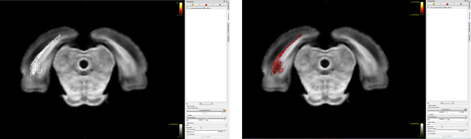
Ah! My bad…I hope it’s better this time  Basically, I want to visualize significant fixels in FDC (pic 1) as streamlines color coded by percentage effect (pic 2) using the .tsf files for percentage effect & p-value. I would expect to see a percentage decrease in the tracts (which I can’t visualize for some reason!). So, I was just wondering if I’m loading the images the right way
Hello all,
I am performing FBA (Fibre density and cross-section - Single-tissue CSD) using the intructions: https://mrtrix.readthedocs.io/en/latest/fixel_based_analysis/st_fibre_density_cross-section.html
I have 4 subjects, 2 controls, 2 patients:
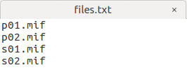
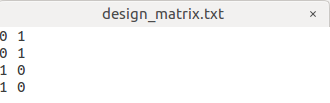
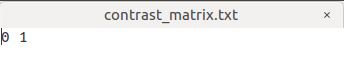
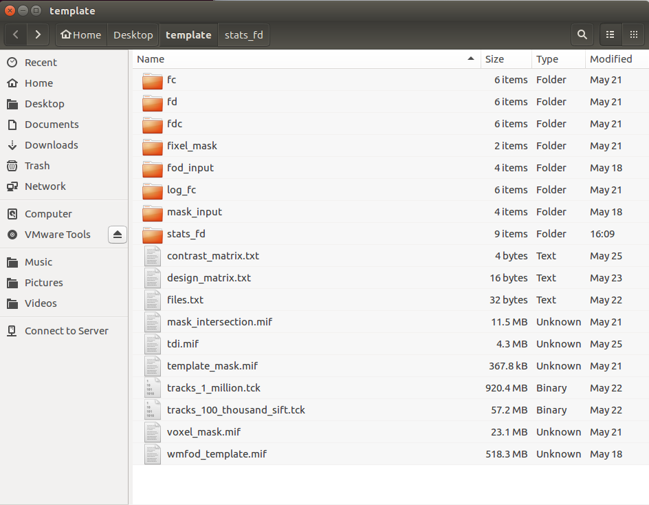
I want to Perform statistical analysis of FD, FC, and FDC as the step 22, my command is:
fixelcfestats fd files.txt design_matrix.txt contrast_matrix.txt tracks_100_thousand_sift.tck stats_fd
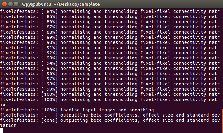
but i get into trouble as follows:
The step of statistical analysis of FD does not seem to have been completed (I’ve been waiting more than two days:disappointed:),.
Do you have any ideas of what could be wrong?
Regards,
Pinyi Wang
Hi @PinyiWang,
The fixelcfestats can be pretty taxing on your system in terms of CPU usage, but more importantly: memory requirements. As it’s still running at this stage, how is your memory usage (and swap space usage) going on your system?
Also, since the memory requirements are so particularly high for this, definitely make sure that anything else requiring (a lot of) memory is shut down… That would e.g. include browsers and programs that load a lot of data (e.g. Matlab with a large workspace, etc…) in particular. But anything that’s using a lot of memory in general really.
Cheers,
Thijs
Thanks for your response.
My system is ubuntu 16.04 on the VMware Workstation, 24GB of memory, 8 CPU, 300GB hard disk space.
Maybe that is not enough for the usage of fixelcfestats…
Regards,
Pinyi Wang
Yes, I’m not 100% sure, but I wouldn’t be surprised if you ran out of memory and the process started swapping. It won’t crash immediately, but it may start to take forever essentially, to either eventually (after a few years; not kidding) finish, or still crash because all the swap space is gone as well.
The only way to be really sure that this is the issue, would be to check the memory/swap state of your system after having it run for at least a good day (24 hours) or so. By then, it would become clear whether it’s hitting the limits of your RAM memory or not.
OK, i will check the memory of my system after having it run for 24 hours.
Perhaps I should buy a new system…
Thanks again for your reply.
Regards,
Pinyi Wang
That’s probably going to end up being the solution indeed. For a typical fixel-based analysis, where you would e.g. have up to 500000 fixels, you need 128GB of RAM to be able to run such a thing. The memory requirements scale roughly quadratically in function of the number of fixels (and as we our discovering ourselves – live – over here, a number of other things further influence this). Even with 64GB of RAM, it may be hard. Rather than potentially investing a lot of money in hardware, it may be worthwhile exploring availability of a cluster at your institute, or institutes that you know in your community; unless you’re expecting to do this kind of analysis very routinely, and want to explore a lot of different designs, etc…
Yes, our computer cluster platform is under construction right now…Hope it can be finished as fast as possible…
Anyway, thanks for your advice!!!
Regards,
Pinyi Wang
No worries; you’re welcome!
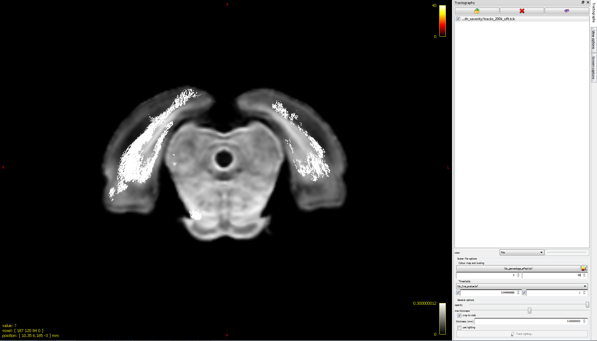
I would expect to see a percentage decrease in the tracts (which I can’t visualize for some reason!).
There are a couple of things that would be worth looking at here:
In the lower image, you are setting the colour bar range from 0 to 40. However from the relevant documentation page, there are two different equations provided; the first is relevant for FDC and includes multiplication by 100 to get a genuine “percentage”, whereas the second is relevant only for FC and does not include that multiplication step. Make sure you have used the first equation.
The example makes certain assumptions about the structure of your design matrix and the arrangement of factors within it, since it directly reads from image beta1.mif. Therefore you need to cross-check the actual mathematical operation this example is performing with your actual experiment and ensure that it is an appropriate expression.
You should also check the sign of the effect and any derived calculations thereof.