OK, this seems to kinda work. It’s not the same approach as in the paper mentioned, but I think it’s a broadly similar idea. The main difference is it takes out the CSF contribution from the raw DWI signal, rather than computing both the CSF fraction and tensor elements jointly. In my opinion, this makes it more general since you end up with the CSF-suppressed DWI signal, which you can process however you want – but the disadvantage is that downstream processing will probably become unstable in regions where there is no longer much signal – as you’ll see from the screenshots below.
The main idea is:
- use MSMT CSD to obtain the CSF fraction
- forward-model the CSF fraction to generate its predicted signal in the DWI
- subtract this from the original DWI
Here’s what the commands looks like:
# Get response function for MSMT-CSD:
dwi2response dhollander dwi.mif -mask mask.mif wm.txt gm.txt csf.txt

# Perform MSMT-CSD fit
# If data are single-shell, drop the last two arguments to omit the GM from the MSMT CSD fit:
dwi2fod msmt_csd dwi.mif -mask mask.mif wm.txt wm.mif csf.txt csf.mif gm.txt gm.mif

# Forward-project CSF fraction onto DWI
# Here, we need to remove the DW scheme from the final CSF signal image header,
# otherwise it can mess things up later on:
shconv csf.mif csf.txt - | sh2amp - dwi.mif - | mrconvert - -clear dw_scheme dwi_csf.mif

# Subtract CSF signal from the original DWI:
mrcalc dwi.mif dwi_csf.mif -sub dwi_fwe.mif
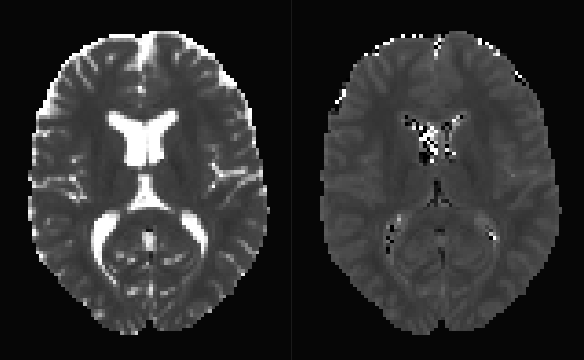
Here’s what this produces on some test data. As you can see, the DTI fit becomes unstable in CSF regions. Not sure if that’s what you were after…
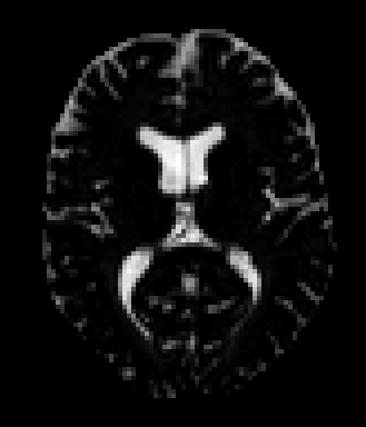
Estimated CSF fraction:
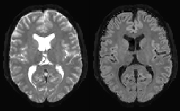
b=0 volume:
left: original; right: with free-water elimination
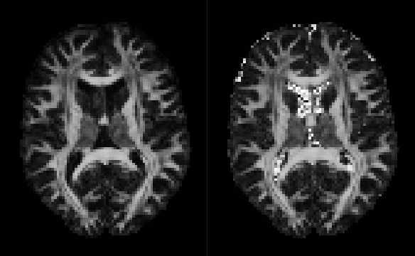
FA map:
left: original; right: with free-water elimination
MD map
left: original; right: with free-water elimination