Free water compartment analysis

Dear MRtrix3 team and users,

I’m interested in splitting the diffusion contribution in two: the free water compartment and the tissue compartment, as suggested by these two papers: doi 10.1002/mrm.22055 and doi 10.1016/j.jalz.2017.12.007.

I was just wondering if is there any commands related to it in MRtrix3.

Cheers,
Andre

Funny, I’ve just had recent conversations about precisely this…

Short answer is: I think we can do something that approximates this very well relatively easily. I’d need to work out the exact sequence of commands though, but it shouldn’t be too difficult.

Give me a minute to work this through, I’ll update once I have something.

OK, this seems to kinda work. It’s not the same approach as in the paper mentioned, but I think it’s a broadly similar idea. The main difference is it takes out the CSF contribution from the raw DWI signal, rather than computing both the CSF fraction and tensor elements jointly. In my opinion, this makes it more general since you end up with the CSF-suppressed DWI signal, which you can process however you want – but the disadvantage is that downstream processing will probably become unstable in regions where there is no longer much signal – as you’ll see from the screenshots below.

The main idea is:

  • use MSMT CSD to obtain the CSF fraction
  • forward-model the CSF fraction to generate its predicted signal in the DWI
  • subtract this from the original DWI

Here’s what the commands looks like:

# Get response function for MSMT-CSD:
dwi2response dhollander dwi.mif -mask mask.mif wm.txt gm.txt csf.txt

# Perform MSMT-CSD fit
# If data are single-shell, drop the last two arguments to omit the GM from the MSMT CSD fit:
dwi2fod msmt_csd dwi.mif -mask mask.mif wm.txt wm.mif csf.txt csf.mif gm.txt gm.mif   

# Forward-project CSF fraction onto DWI
# Here, we need to remove the DW scheme from the final CSF signal image header,
# otherwise it can mess things up later on:
shconv csf.mif csf.txt - | sh2amp - dwi.mif - | mrconvert - -clear dw_scheme dwi_csf.mif

# Subtract CSF signal from the original DWI:
mrcalc dwi.mif dwi_csf.mif -sub dwi_fwe.mif

Here’s what this produces on some test data. As you can see, the DTI fit becomes unstable in CSF regions. Not sure if that’s what you were after…

Estimated CSF fraction:

screenshot0000

b=0 volume:

left: original; right: with free-water elimination
screenshot0000

FA map:

left: original; right: with free-water elimination
screenshot0001

MD map

left: original; right: with free-water elimination
screenshot0002

2 Likes

Great. It might work for my purposes. Thanks a lot, Donald.

Best,
Andre

Hi @jdtournier,

I’m interested to try this approach in my dataset (neonatal data), however I don’t have the last mrtrix version (I have the version 3.0_RC3-15-g9494da8d), so I have to edit some of the commands:

mrconvert input.nii.gz dwi.mif -fslgrad bvec bval -export_grad_mrtrix grad.txt
dwi2response dhollander dwi.mif -mask mask.nii.gz wm.txt gm.txt csf.txt -fa 0.1 -voxels voxels.mif
dwi2fod msmt_csd dwi.mif -mask mask.nii.gz wm.txt wm.mif csf.txt csf.mif
shconv csf.mif csf.txt - | sh2amp - -gradient grad.txt - | mrconvert - -clear_property prior_dw_scheme dwi_csf.mif

But when I do the final step: mrcalc dwi.mif dwi_csf.mif -sub dwi_fwe.mif

It shows the following error:

mrcalc: [ERROR] dimensions of input images do not match - aborting

The dimensions are 128 x 128 x 56 x 153 (dwi.mif) and 128 x 128 x 56 x 64 (dwi_csf.mif), I think the problem is in the sh2amp command (because in this version I can not put an image to sample to the same directions), is there any work around to solve this, without updating to the most recent version? Thanks in advance.

Best regards,

Manuel

Yes, unfortunately you’ll need these changes to shconv and sh2amp, which are only available in 3.0.0. The main issue is that both commands were only capable of handling single-shell data till now.

This can probably be done using older versions, but it would require a lot of scripting and massaging to handle each shell in turn and recombine into a coherent DWI data set – and the b=0 volumes will probably need to be handled separately as well. I personally wouldn’t recommend it. But you can always install 3.0.0 alongside your main installation if that helps…? Recent discussion on this topic here.

Hi,

Thanks for you reply, I will do that.

Best regards,

Manuel

Thanks for sharing this code @jdtournier!

I’m new to using Free Water Compartment Analysis and have a question about csf.mif. If the normalised CSF FOD is available (obtained using mtnormalise, and also generated using the group average response function) would it make sense to replace csf.mif with the normalised CSF FOD?

Cheers,
Arkiev

Hi Arkeiv,

Good question! It might, but only if you’ve also corrected the bias field estimated via mtnormalise to the DWI images. For that, you’d need to get mtnormalise to also output the field via the -check_norm option, and then use mrcalc to multiply the DWI by that field. I think that ought to do it, but note I’ve not tested this in any way!

All the best,
Donald

Hi Donald,

Got it - thanks!

With respect to the Estimated CSF fraction image, is this showing the first volume of dwi_csf.mif? My understanding is that the CSF fraction map should have only a single volume (and have a range from 0 to 1). The dwi_csf.mif that I have computed has more than one volume…do you have any thoughts on the best way to reduce this image into a single volume?

Cheers,
Arkiev

Hi Arkiev,

These are not strictly speaking fractions, but close enough post-mtnormalise… If you’re asking about the scaling, it won’t between 0 & ~1 primarily because these are expressed in spherical harmonics, so a DW signal amplitude of 1 equates to a l=0 term of value 1/√4π.

As to dwi_csf.mif, I assume you’re referring to my original instructions? In which case, that file should correspond to the expected CSF signal for the DW scheme included in the dwi.mif header, assuming CSF density (~ “volume fraction”) in csf.mif.

Does that answer your question…?
Cheers,
Donald.

Hi Donald,
Ah okay, noted - thanks for the explanation!

Yes, I was referring to the original instructions, in particular, this image:
CSFfraction

Is this image dwi_csf.mif? It looks like a CSF map, but as you said, it isn’t really a fraction…

I think there might be a simpler solution for what I am after, but I am not sure if it is analogous to measuring “free water”. CSF_norm.mif is a 3D volume, and can be further normalised by dividing by it’s maximum value. The resulting image will have a range from 0 (i.e., no CSF-like material) to 1 (completely CSF-like material).

Does it make sense to say that, at least in this context, the fraction of CSF-like material is the fraction of free-water? :thinking:

Thanks for your time!
Arkiev

No, that’s the csf.mif image - which is the estimate of CSF “density”. As I mentioned earlier, after mtnormalise, it is close to a fraction, but scaled between 0 & 1/√4π (because it’s expressed as the l=0 SH coefficient), but not strictly so (it can go above that value, since mtnormalise doesn’t constrain the estimated densities to sum to 100% (i.e. 1/√4π), only that (after correction for the bias field) the sum of the estimated densities averages to 100%.

You could normalise the csf.mif image more explicitly as you suggest, but you will then tend to underestimate your CSF fraction since any noise in the estimated densities will produce more extreme maximum values. I wouldn’t personally recommend that.

Indeed, this is where the distinction is going to get a bit cloudy… In my mind, CSF is the closest thing to “free water” in the brain. But if you’re looking for something that estimates “free water” in the tissue, then we need to distinguish between water in the extracellular space (which can be viewed as “free” in that it is not constrained in the sense that the intracellular water is), and water that genuinely diffuses freely – which won’t generally be the case for extracellular water in healthy brain tissue, since the motion of water molecules will definitely be influenced by the cellular environment (axons, glial cells, etc).

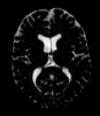
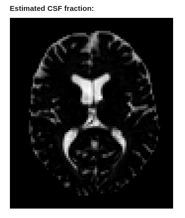
The way the technique I’ve suggested works assumes you’re after water that can genuinely be considered to be diffusing freely, since its signal properties are assumed to match that of CSF. In general, that probably won’t capture extracellular water in the tissue. In fact, you can easily see that it doesn’t by looking at that csf.mif image itself: it will have close to zero “density” in most of the parenchyma, which doesn’t tally with estimates of 20% extracellular space that you will see in the literature.

In fact, if you really think about this, you’ll see that for healthy tissue, the extracellular water is actually already captured in the response function for each (non-CSF) tissue type. The WM response is measured from voxels assumed to be 100% occupied by WM, and their signal is used as-is as the response. The densities we obtain correspond to those that match that specific “signature” - including all of the different compartments that contribute to its signal.

As a side note: this may sound counter to the interpretation often suggested in the literature, which is that the WM odf provides an approximation to the intra-axonal water fraction, based on some of our early work. That’s because that early work only applies to single-shell CSD at high b-value – under those conditions, then yes, the odf ought to provide an estimate of the intra-axonal water (assuming healthy axons). But the analysis we’re talking about here is explicitly multi-shell, and as such, the signal at low b also contributes to the fit – and that signal will definitely contain extracellular contributions. In this context, the response functions will represent the signal you’d expect for that tissue type as a whole – including its intra and extra cellular contributions. And yes, the intracellular contribution will dominate the high b aspects of the response, but there will nonetheless be extracellular contributions in the low b range.

I guess part of the problem is I don’t know what you’re after exactly… :stuck_out_tongue_winking_eye:

Cheers,
Donald

2 Likes

Is this purely because of noisy voxels? And if so, as a workaround, could the output of mrthreshold be used as the normalisation factor (instead of using the maximum value)? And subsequently, replace values greater than the threshold with 1?

This is what I would like to measure :grin: although, going one step further, I would like to generate a single-volume 3D map (scaled from 0 to 1) of free water fraction (and eventually, measure the average free water fraction in GM and WM tissue).

Thanks for pointing this out…to potentially add a layer of complexity, the data I am working with is single-shell (b=0,1000), and has been processed using single-shell 3 Tissue (mrtrix3tissue)… does this have any implications on the interpretation of the measurement? :thinking:

Again, thanks for the insightful responses - greatly appreciated!
Arkiev

Yes, mostly.

Not sure I follow that logic… The problem is that if you decide to normalise by the maximum value, it will typically come out considerably larger than expected – we just need to avoid undue influence from these large maximum values. The output of mrthreshold has no guarantees of being anywhere near the right value. But more to the point, we know the normalisation factor is 1/\sqrt{4\pi}, so I would recommend just using that – more on that in the next point.

OK, based on that, I would suggest that your best bet might be to multiply the csf.mif (after mtnormalise) by \sqrt{4\pi}, and clamp to 1. Something like this:

mrcalc csf.mif 4 pi -mult -sqrt -mult 1 -min csf_vf.mif

which performs this operation:

mrcalc: [100%] computing: min ((csf.mif * 3.54491), 1)

OK, it will change the values you get to some extent (depending on a number of factors), but in my opinion that’s independent of the interpretation. SS3T is still ‘multi-shell’ (it relies on the b=0 signal), so the same logic applies as in my previous post.

Cheers,
Donald.

1 Like

This is incredibly helpful - thanks Donald!!

Cheers,
Arkiev