How to estimate an ideal Response Function for an ex-vivo spinal cord

[ihattan]

Dear Mrtrix Experts,
I have an ex-vivo human spinal cord dataset. They are with 2 bva0 and 750, and 1500, each 12 directions. I’m trying to get a good response function in order to generate CSD map and Tractography. I would like to use Mrtrix 3 to do so.
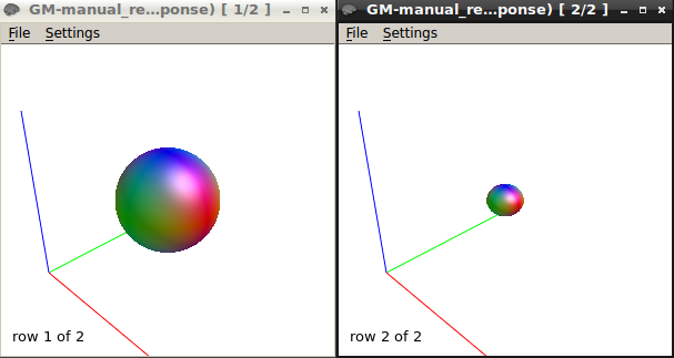
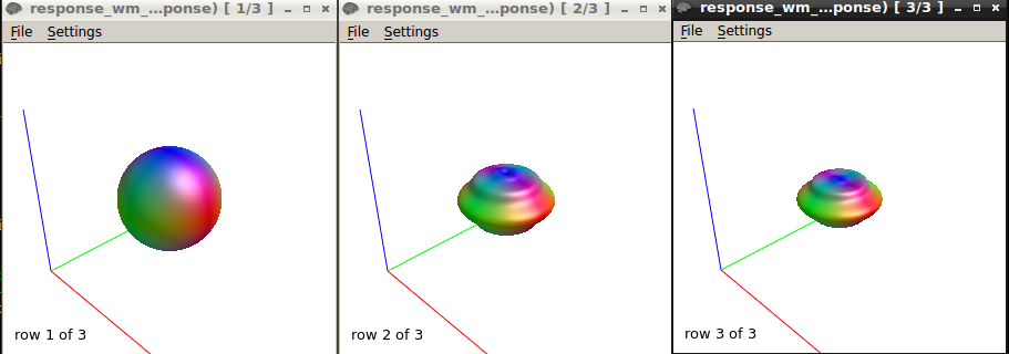
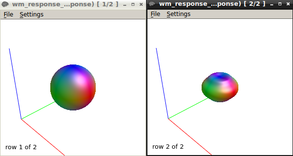
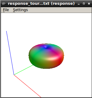
I’ve used the dwi2response tournier , dhollander, fa and manual algorithm using the whole cord or only selecting for the single fibre orientation WM tract areas. I am still not satisfied about the outcome of response function. I think I should aim to get a response function close to a flat oblate shape in order to get a good FODs? Could you recommend if this can be better performed?
I have done the following steps:
A. response calculation using the whole cord mask

1. I converted the dicom to nifti format using (MIPAV) for first sample 3 shells b0,750 &1500. For second sample (b0&3000) I used mrconvert dwi2nifti

2. For the gradient table, I swapped the gradient from xyz to zyx (I used data that come from Bruker preclinical animal scanner)

3. Biasfield correction of the B0 using ANTS N4biascorrection, and applied this correction to the whole 4D DWI dataset

4. Then, I ran the following tests for each individual shell

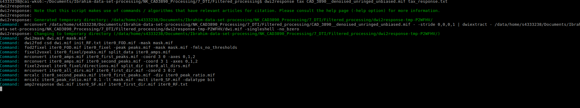
A-Response function calculations using the “tournier” algorithm using a mask containing whole cord at b-value 1500

dwi2response tournier < Input DWI> < Output response text file>

The above commands were repeated for the b=750.

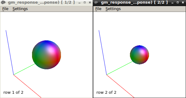
I got this response function at b1500.

The response function values at b1500 are
16616.92061510039 -3585.731063681506 662.1366725620043 -49.21846975544766 -372.193208900446 89.22703866558832

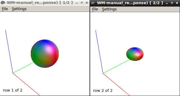
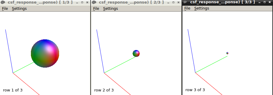
Also, I tested the TOURNIER algorithm on another sample with 2 shell (b0&3000). I got the following response function

The response function values at b3000 are 15261.69894075049 -3513.609487088777 1043.844357488741 -145.3679829867056 2.01888135870964 11.80721638417216

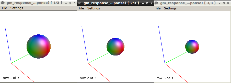
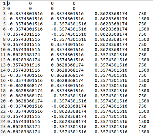
B-Response function calculations using the “tournier” algorithm using a mask containing selected voxels of SPINAL CORD WM AT b-value 750 & 1500

The response function values at b750 are
24174.5778079981 -1711.70084036846 442.5087763272201 13.27346114028632 12.25772995997397 -58.66570209134966

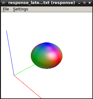
here is the response function using the same algorithm at b1500

The response function values at b1500 are
9416.77124310872 -1993.300817125692 211.8305534782687 85.78772928903967 -89.50880832164782 54.91400798555078

*The other methods for response function result will be posted soon.

Many Thanks,

Hattan

[ihattan]

Related to the main topic so here are the rest of the other algorithms

C- Response function calculations using the “Manual” algorithm using a mask containing selected voxels of SPINAL CORD GM & WM AT b-value 3000
I ran this command

dwi2response manual

The response can be seen on the following figure GM and WM
1-RESPONSE OF GM

The response function values of the GM at B3000 are
39275.36715467063 0 0
13212.79354595523 -657.8615146152904 75.63832341624993
2-RESPONSE OF WM

The response function values of the WM at B3000 are
33147.83258401395 0 0
18104.61783172658 -1810.264217250323 334.2830248917984

D-I tried also testing Tax algorithm using whole cord with the following command

dwi2response tax dwi_denoised_unringed_unbiased.mif tax_response.txt
However, I tried to run Tax algorithm for several times on multiple samples with no respones for any outcome. I wait over 24hours and the following screenshot shows the progressed steps

E- Response function calculations using the “dhollander” algorithm using a mask containing whole cord AT b-value b0, 750 & 1500
*GM response and values

*Values are
35120.56308613496
25970.16274180858
20351.72473768609
*WM response and values

The response function values are
84721.78164399209 0 0 0 0 0
63440.44453727814 -8336.822253691626 1468.938157010697 -1109.758004909964 1483.118442704632 -1435.678812917911
52254.21406727003 -9746.011375347643 1282.457947363209 -828.1941963688256 2081.772088686 -1235.936454682478

*CSF response and values

*values
41178.56309785594
10338.79280139325
3014.292512204908

*The gradients table used for the 3 shells 0,750&1500 as shown below

*I also tried to run the the “dhollander” algorithm using a mask containing whole cord AT b-value b0, 750 to see if there are any differences and may get a good Response Function so the results as shown below
*GM response and values

35154.62085839952
23123.96888811249

*WM

The response function values are
28522.00201983786 0 0 0 0 0
20103.85596097083 -2276.156972952893 -26.24608254976766 -542.9209838387386 100.6540617084113 168.1171227640265
Then I repeated at b1500 as seen below
*GM output and values

*values
35154.62085839952
23123.96888811249

[jdtournier]

Wow, that’s a lot of work…

Unfortunately, I have no experience at all with spinal cord… I’m guessing a large part for the instability in these responses will be due to the low number of voxels that are eligible in the spinal cord, so you might end up with either very few voxels included, or conversely for some estimators, too many voxels, including some that really aren’t appropriate as single-fibre exemplars…

So my suggestion would be to persevere with the manual method – at least you can control which voxels are used to estimate the response function. But for some reason, yours were only estimated up to l_max=4, which is unexpected – it should default to l_max=10. Did you manually specify this? What does it look like if you allow it to use a higher value (e.g. 6 or 8)?

Also, I’m not sure what the response should look like in the spinal cord, but you’ll probably find that you get reasonable FODs even if the response is a bit funny-looking. As long as it has the right overall shape, it should still pull out reasonable orientations from the data… Have you actually tried seeing what the FODs look like? However, whether this is good enough will ultimately depend on what you plan to do with the data, whether strict quantification will be required, etc.

[rsmith]

For the gradient table, I swapped the gradient from xyz to zyx (I used data that come from Bruker preclinical animal scanner)

In addition to the above, you need to be absolutely confident that your gradient table is correct; when it’s not, response function estimation is the first thing to go awry. The dwigradcheck script might work if you provide it with a good mask. Alternatively, use the mrview ODF tool, loading the DWI data into the toolbar. This allows you to visualise the DWI data directly. You will likely have to play with the “Scale” setting in the toolbar in order to change the size of the resulting glyphs to something reasonable. You want to make sure that in the WM of the cord, the approximately pancake shape of the DWI signal curves spatially in accordance with the orientation of the cord.