Low b-values with increasing and decreasing response function magnitude

[Alistair_Perry]

Hello,

I have acquired a diffusion sequence containing a small number of diffusion-weightings at b 500 (n=10) and b 200 (n=6), for free-water estimations outside of MRtrix. The other embedded shells are the now standard b 1000 (n=20) and b 3000 (n=60) weightings.

Upon viewing the response function estimations with the following code:

dwi2response msmt_5tt dwi.mif r5TT.nii wm.txt gm.txt csf.txt -mask brainmask.nii

I noticed that the response function values for the white-matter derived tissue, within each row, are not decreasing in magnitude. The b 1000 shell on later inspection (fourth row), demonstrate values that appear strangely problematic.

To note, the slm-linear option has been passed onto dwipreproc.

However, when I choose only to include the b 1000 and b 3000 shells for analysis, through setting -shells 0,1000,3000, this issue appears to be slightly circumvented:

And when using dhollander:

dhollander, now with only the b 1000 and b 3000 shells, which is more stable:

I presume that the response function estimation is not optimal with a smaller number of vectors? Moreover, if I were to be using this data for MRtrix-alone purposes (i.e. connectome generation and/or fixel-analysis), it’s perhaps best that I remove these sub-b1000 shells?

I did create this diffusion vector set using an older version of gen_scheme, which is illustrated below:

Statistically checking the metrics of the current diffusion vector set does indicate the directions of the sub b 1000 shells are “asymmetric”.

(b=199.99998408333332) [ 6 directions ] 

 Asymmetry of sampling:
    norm of mean direction vector = 0.210423

(b=500.0000467000001) [ 10 directions ]

  Asymmetry of sampling:
    norm of mean direction vector = 0.101242

The full report is attached here

Some basic quality checking of the diffusion signal across the shells:

b200:

b500:

b1000:

b3000:

[maxpietsch]

@Alistair_Perry

I noticed that the response function values for the white-matter derived tissue are not decreasing in magnitude. The b 1000 shell on later inspection (fourth row), is strangely problematic.

The first column represents the mean signal in each shell, which is decreasing, the other columns contain the higher order (zonal) harmonic coefficients. You can use shview -response to render your response functions. You should see a sphere that flattens with increasing b-value. See this paper for more details.

[Alistair_Perry]

Thanks @maxpietsch,

As expected, the harmonic profiles do flatten with increasing b-values:

Although, I believe you slightly misinterpreted my question. My concern is that across the rows within the response function (particularly for the fourth column), the values are not decreasing in magnitude.

To re-demonstrate:

1424.338561611295 0 0 0 0 0
1225.505145912768 -113.8049914665067 5.926890244010404 12.14004544561863 -1.987244138897725 -0.1513613190009629
996.4274607021107 -223.4550228077395 25.92133803121068 -1.706167904058339 2.894367009973647 -2.416315779943908
755.7359056395113 -294.244980880778 60.54861123526116 -9.801876577539458 0.8006653524501117 -3.040617336570455
425.0788579985894 -263.739174182725 128.6349007503337 -45.63362162755784 10.94698263203365 -2.881451573447199

This is unexpected to what I normally obtain with standard one- or- two three shell acquisitions, and oppose what @jdtournier notes within the legacy MRtrix2 documentation.

Perhaps @jdtournier, @ThijsDhollander you could provide some assistance here - albeit I know you guys are very busy with the upcoming workshop!

Best,

Alistair

[rsmith]

Hey Alistair,

So, a couple of different things to disentangle here.

amp2response

The “golden rule” of having zonal spherical harmonic coefficients decreasing in magnitude (and flipping in sign) with increasing harmonic degree came about from long-term observations of the behaviour of response function estimation, dating back as you say to the old 0.2 version of the software, and makes sense given the expected “pancake” shape of the response function and the reduced signal power in higher harmonic degrees.

This was however based on older methods for estimating a response function from a set of voxels deemed to be “single-fibre”, and the estimated fibre directions in those voxels. The old estimate_response command, as well as the MRtrix3 command sh2response, operate as follows:

• In each single-fibre voxel:

  • Rotate the DWI signal on the sphere, in such a way that the estimated fibre direction lies along the z-axis.

  • From the full spherical harmonic representation of the rotated DWI signal, discard all m!=0 components.

• Average the m=0 coefficients across all single-fibre voxels.

Since 3,0_RC3 however, the script algorithms within dwiresponse have been using the new command amp2response (GitHub discussion here; method abstract here). This uses the information from all single-fibre voxels in a single determination of appropriate response function coefficients.

There are two crucial discrepancies here:

• The amp2response method additionally enforces non-negativity and monotonicity of the response function. The response function coefficients are necessarily modified in order to enforce this constraint.

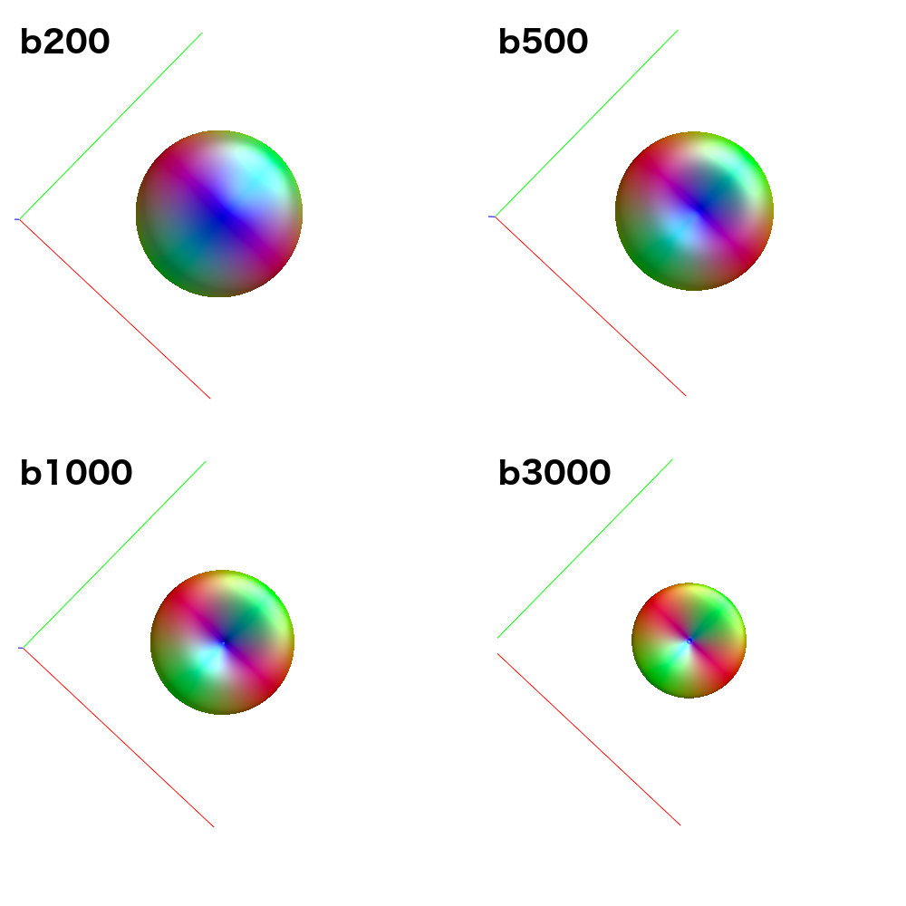
• Because it uses data from all single-fibre voxels at once, amp2response can fit a higher harmonic degree than what would have been possible previously. For instance: Your b=200 shell contains 6 volumes; enough for a lmax=2 fit. Previously, this would have meant estimation of a response function with only 2 non-zero coefficients for this shell. amp2response in comparison is providing an lmax=10 response function, despite having only 6 volumes. So while the coefficient magnitudes are not monotonically decreasing, they were in fact previously unattainable.

Now having described that, I’ve no guarantee that estimating and using such high-degree coefficients for low-b shells is actually beneficial; as I flagged in the original GitHub discussion around its inclusion, this may at the very least come off as “unusual” to users, but I’ve never actually had such data in order to test the effect of inclusion of those coefficients (bearing in mind that in the initial transformation of DWI data to SH coefficients for CSD, the SH coefficients of the data in those higher degrees will necessarily be zero). If you felt so inclined, you could experiment to see what kind of response functions you get:

• Using sh2response instead of amp2response

• Using the -noconstraint option in amp2response

• If you really want to get your hands dirty, uncomment this line and re-compile…

Using different shells in dwi2response

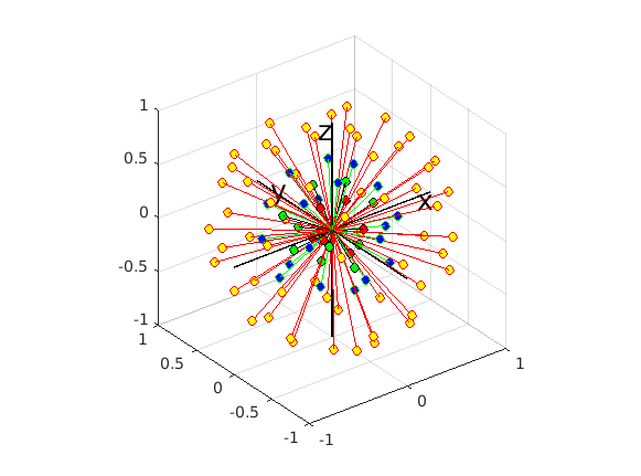
Here I need to be very clear in differentiating between the different steps in processing: While amp2response is responsible for taking a pre-determined set of single-fibre voxels and estimated fibre orientations and producing the response function coefficients, the major task of the various dwi2response algorithms is the selection of those single-fibre voxels.

Now I should clarify that given reducing your data to only the b=0;1000;3000 shells, the resulting response function coefficients should correspond to the first, fourth and fifth rows of those obtained when all shells were used. So when you look at the data appropriately, i.e. omitting the second and third rows from the full data results and then comparing to b=0;1000;3000 data, they are in fact very similar. There’s maybe a little numerical discrepancy, which could be due to imprecision in the numerical solver utilised within amp2response, or it could be due to selection of a different set of voxels for response function estimation…

The question then is whether dwi2response msmt_csd or dwi2response dhollander may select a different subset of voxels for response function estimation of each of the three tissues.

• dwi2response msmt_5tt involves calculation of FA, which is in turn used to refine selection of GM and CSF voxels. But estimation of the WM response function specifically shouldn’t be affected.

• dwi2response dhollander can really only be clarified with certainty by @ThijsDhollander; I thought it had been commented that it only uses b=0 and the highest b-value shell, but from the current code it seems to be doing some operation over shells, which means the outcome could conceivably change if certain shells are omitted from the data. But I’m fully waving the ignorance flag here.

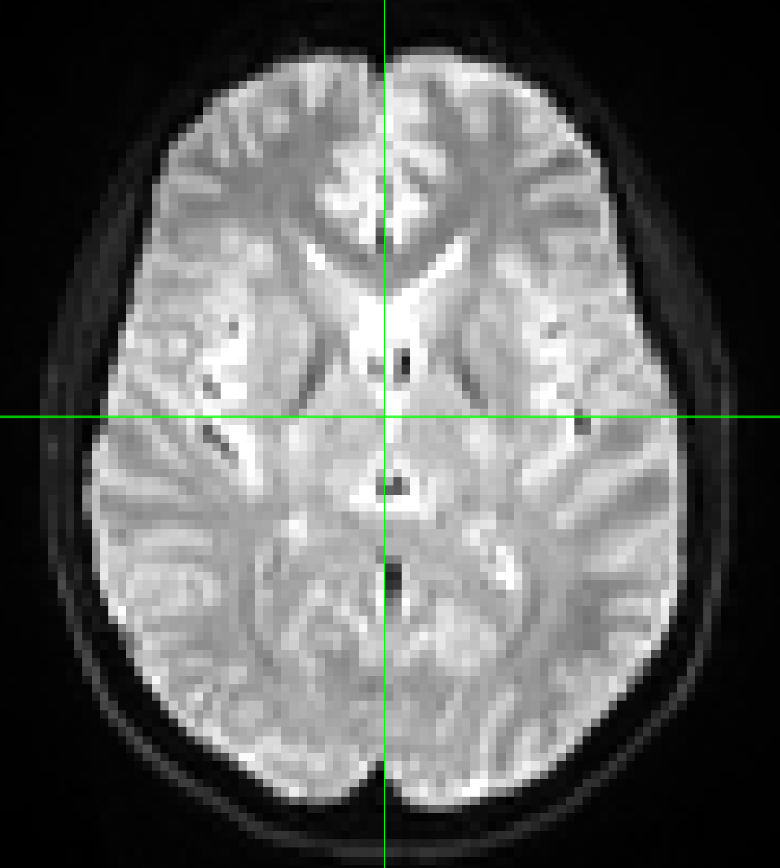
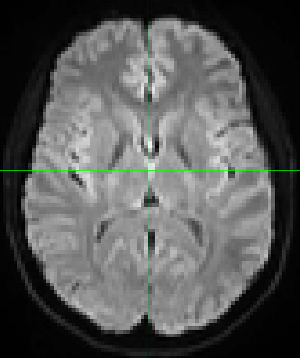
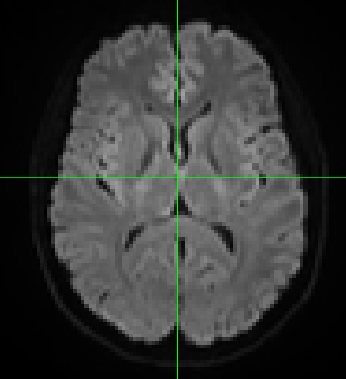
As mentioned above, it’s possible for there to be some imprecision in the solver used by amp2response, so reporting only variation in those coefficients is not enough information to tell exactly where the variation in results is coming from. So it would be worthwhile using the -voxels option in dwi2response to see whether or not the selection of exemplar voxels is in fact changing.

---

Rob

[jdtournier]

Just adding my 2 cents to what @rsmith has already said:

As @rsmith mentioned, the rule that response function coefficients should be decreasing in magnitude as a function of harmonic order was always purely based on observation – there is no formal proof for this that I’m aware of…

Looking back at your problem, rows 2 & 3 correspond to b=200 & b=500 respectively, which I’d expect to contain little or no power in the higher harmonics (certainly nothing much beyond l=4 – 3rd coefficient). But they get estimated anyway nowadays because amp2response works differently, as @rsmith explained. But it doesn’t mean they are significant: there is noise in the data, and typically quite a lot of it at low b-values, particularly in or near the ventricles (maybe due to CSF flow or pulsation, I’m not sure, but it does look physiological rather than thermal in origin). The only other problematic entry is the last one on row 4: l=10 at b=1000 – again, I’d expect that coefficient to be negligible at that b-value, and certainly dominated by noise.

Thankfully, if you look at the most problematic coefficient on row 2 (4th entry), it’s still <1% of the mean signal at that b-value. The other coefficients are smaller still. So I’m not sure there’s any conclusion to draw from that other than higher harmonic coefficients at low b are dominated by noise…

---

Otherwise, just to clear up any potential misunderstandings:

@rsmith

bearing in mind that in the initial transformation of DWI data to SH coefficients for CSD, the SH coefficients of the data in those higher degrees will necessarily be zero

There is no initial transformation to SH in our implementations of CSD (other than maybe for the initial solution). All SH coefficients up to the requested l_max (8 by default) are used to compute the forward model for the DW signal, and that matrix is used in the constrained fit. Note that this makes no difference to what @rsmith was saying, it’s just me being pedantic…

[ThijsDhollander]

@jdtournier

So I’m not sure there’s any conclusion to draw from that other than higher harmonic coefficients at low b are dominated by noise…

Hi @Alistair_Perry,

Essentially, @jdtournier (see quote) is right here, and there’s no immediate reason for concern. However, there’s a few potential additional reasons why this may arise from the current algorithms, especially the mechanism many of them share to select the single-fibre white matter response function. Still not a big concern, but there’s some room for improvement indeed (although I doubt that would ultimately be the explanation/“solution” to the non-decreasing coefficient magnitude you observe; that in and of itself is probably not even a problem to begin with). I’m looking into this currently, with a few solutions in place even, although their robustness remains to be tested at my end. I’m not one to sacrifice robustness over some accuracy in all cases… so well, I’ll see what the testing gives. @Alistair_Perry, if you’re really concerned for your particular application or project, happily be in touch. I’m already trialling some changes in a few projects with external collaborators; but of course safely supervised at this stage.

@rsmith

dwi2response dhollander can really only be clarified with certainty by @ThijsDhollander; I thought it had been commented that it only uses b =0 and the highest b -value shell,

Well, certainly not commented by me, that would be.

@rsmith

but from the current code it seems to be doing some operation over shells, which means the outcome could conceivably change if certain shells are omitted from the data.

Oh yes, of course. The algorithm leverages as much of the data as it can, all within Occam’s razor’s principles of course (no need to try and get from the data what isn’t in there). All clearly documented in the original abstract. Also, if people are still wondering, here’s some additional insights on how msmt_5tt and dhollander perform with respect to each other. So far, that pattern has generalised over all data I’ve encountered so far, including ranges of lesions, more lesions (also, we’ve used it in MS studies, and it’s been used internally on a stroke cohort, and externally on a few other pathologies), animal data, ex-vivo data as well as babies. Someone at our recent workshop had single-shell b=800 data with a low number of directions (don’t recall the exact number), with a massive cyst in the brain, and an equally massive MR artefact that distorted part of the brain and basically destroyed the signal in that area… well, dwi2response dhollander still selected sensible voxels. But the message here should always be: check your -voxels output. If it looks sensible, you’re good.

But well, your results will change depending on which b-values you feed into it; that’s entirely expected and by design… no need to worry about that.

[mblesac]

Hi,

Sorry for bringing this topic back to life, but I have a related question.

I have a manuscript under review when we do MSMT-CSD (using dhollander for the response function) with an acquisition that consists in: 16 b0, 3 b = 200, 6 b = 500, 64 b = 750 and 64 b = 2500 s/mm^2. One of the reviewers asked about the potential effect of the perfusion in the low bvalue data (b = 200). My first feeling is that if there is any effect, for this process with these data characteristics it should be insignificant, but I would like to ask your opinion. Thanks in advance.

Best regards,

Manuel

[jdtournier]

Wow, that’s an interesting question!

I can’t see that it can make a lot of difference, given that the IVIM signal is pretty small in the first place, and probably mostly gone by b=200 (I think it’s best observed in the b=50 range or so?). But it’s indeed difficult to rule out in general – mostly because it’s actually the b=0 images that will contain the biggest contribution. I don’t think this is specific to MSMT-CSD particularly.

However, there is scope with your data to actually see whether you can observe an IVIM signal. Assuming some appropriate value for ADC of the IVIM signal, you could produce an isotropic response function for it, similar to the CSF one, and include that an as additional component in the MSMT-CSD. It would be really interesting to see if you could do combined IVIM+dMRI analysis that way…