Hi Ana,
I transferred your question over to its own thread, since the requisite answer strays away a bit from the title of the original thread.
Can you elaborate on the conflation between the fixel-wise FD measure and the WM density image?
I maybe mis-used the word “conflation” there. The intended point is that “the WM density image”, being the l=0 term of the spherical harmonic representation, and the fixel FD values, are not on the same scale. For a voxel that contains a single fibre population, of the same density as those voxels used to determine the response function, the value of FD for that fixel will be 1.0, but the value of the l=0 term will be ~ 0.282. This is due to the choice of normalisation of the spherical harmonics basis that was chosen for MRtrix. The ratio between them is precisely 1/sqrt(4pi). It just means that any time raw numerical values are reported, it’s important to know which of these two the values were derived from.
Just confirming, that will give us the FD for each subject, right?

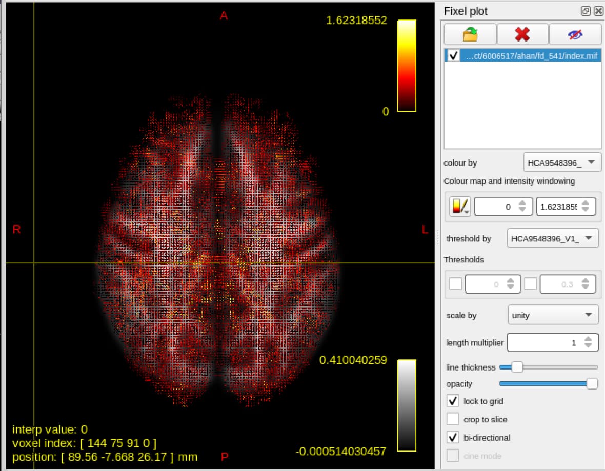
We’re having a similar issue/finding where we get FD > 1 … How do we interpret these fixels with FD > 1?
This concept is something that we should perhaps do a better job of in the documentation. We get the chance to elaborate on it more during the workshop, but haven’t produced static content intended for the wider audience. @Dave wanted to write a whole manuscript on it back in the day, but it got too complicated… 
The key distinction here is the difference between a compositional model and a non-compositional model.
Compositional
- Preeminent example: FSL’s ball-and-sticks.
- The sum of the multiple intra-cellular compartments, and the extra-cellular compartment, is precisely 1.0.
- The signal fraction of any individual compartment cannot exceed 1.0.
- T2 variations may result in different compartments having attributed to them more or less of the DWI signal, with concomitant changes to the other components as their sum must be 1.0.
Non-compositional
- Here considering multi-tissue CSD
- Almost, but not quite, a linear transformation of the data (the non-negativity constraint is non-linear)
- The optimisation finds the right linear combination of the tissue response functions (including anisotropy) that, when put through a forward convolution, recapitulates the empirical DWI data
- Magnitude of any individual tissue compartment is non-negative, but does not have an upper bound.
- T2 variations may result in the affected compartment having more or less DWI signal attributed to it, but ideally the other tissues would not change.
Let’s use an example.
Let’s say that voxel A contains a single fibre population with volume fraction 0.8, and the remaining 0.2 volume fraction is extra-cellular (and I’m pretending here that the PD / T1 / T2 of intra-cellular and extra-cellular water is identical so that I can talk about volume fractions rather than signal fractions). We also assume that the ball-and-stick model is “well calibrated” to the DWI signal, such that it correctly identifies these fractions.
We use voxel A to calibrate our response function for CSD, since it’s the best (only) exemplar that we have. In this particular example, we’re going to use only data from the highest b-value (since it makes the logic easier) If we take that response function, and use it to perform deconvolution on voxel A, we’ll get a single fixel with an FD of 1.0.
Now let’s look at voxel B. In voxel B, the volume fractions are identical to voxel A, but the T2 of the intra-cellular water is drastically longer, such that the DWI signal from that compartment is doubled. If you feed this data to something like ball-and-sticks, exactly what happens will depend on the internal fixed parameters of the model and exactly how the optimiser works, but most likely it will over-estimate the intra-cellular fraction (let’s say 0.9) and under-estimate the extra-cellular fraction (let’s say 0.1). For CSD, you will get an FOD of precisely the same shape, but twice the size; and following FOD segmentation, there will be a single fixel with an FD of 2.0.
So the way that you interpret fixels with FD > 1 is that you have image data where the intensities are larger in magnitude than your “reference” (being your WM response function voxels), and have fed them to a model that does not constrain the tissue composition to sum to 1.0. It just thinks that “there’s twice as much WM” and is agnostic to the fact that the source of the DWI signal is constrained to the volume of a voxel.
In most cases I suspect that it will be due to T2 differences, since the WM response function estimation does not necessarily select those voxels with “the brightest signal”, it also needs to prioritise “single-fibre-ness”. While it’s possible that there may be some voxels where the intra-cellular volume fraction is greater than that of the voxels used to determine the response function, it’s unlikely that they have as much as 1.6 times. In extreme cases it could be due to poor response function voxel selection, or due to having drastically different image intensities across subjects and failing to perform any kind of intensity normalisation. Eg. If you calibrate a response function on a subject where the b>0 DWI intensities are ~ 0.01, and you use that to perform deconvolution on a subject where the b>0 DWI intensities are ~ 100, you’ll get FD values of ~ 10,000. But values of ~ 1.6 are not unusual.
TBH, this issue has been picking at the back of my brain for some time now. We justified the global intensity normalisation approach to ourselves many years ago; but it’s not a clearly superior answer, and it has this common observation of FD > 1.0 that is completely unintuitive to anyone who isn’t a CSD nerd. So can’t guarantee that the recommendations here won’t change in the future…
Cheers
Rob