Quickly checked it using my own simple Matlab script (sorry @jdtournier, but mine has colours and shading and stuff! ![]()
![]() ):
):
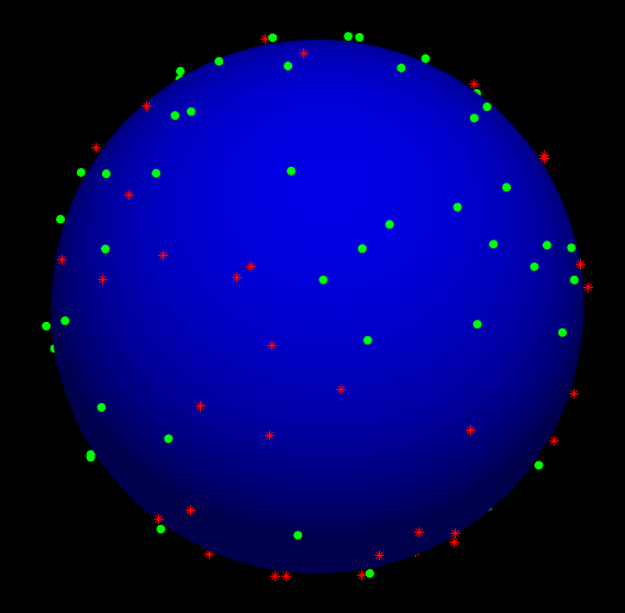
(colours just indicate polarity; green are the polarities in the set, red their opposites)
…so yes, that doesn’t look good at all (and is in line with the findings Donald posted about the set as well). I do expect a bit of mess looking at a single shell, but having used Caruyer’s approach: you’ve got to take into account that that approach tries to optimise the spread per shell, but also across shells (I suppose there’s some weighting between both optimisation criteria). I know some people have started using it in practice… not to be too opinionated, but I’m not sure I’m a big fan of it. It does mess up the sets per shell, and it means that even using 60 directions for your b=3000 shell, you may end up with not enough angular resolution in certain areas of the orientational domain (the big gaps in the visualisation above), and angular biases all over the place. ![]()
…but even using Caruyer’s approach, I find it hard to believe that this would in and of itself lead to the above, if you’ve only got 30 directions on the only other shell. Some of the angles between certain pairs of directions in the set seem so small that you wouldn’t even get them for a 94 direction set (so even just ignoring optimisation within individual shells, and optimising the whole set of 94, and selecting a random subset of 64, would probably not look this bad). The only way I can see this resulting from anything, is using that approach for more than those two shells, and then afterwards just using only the b=1000 and b=2500 shells from it. But that would indeed just be bad practice, and even your multi-shell data at hand is then practically unusable. ![]()
Yep, I can confirm this. It’s the squares of the (L2) norms of your vectors that must scale like the b-values, with the highest b-value just having a unit norm (and then setting that as the b-value of your scan). So for example for a multi-shell acquisition with b-values = 0,1000,2000,3000 your diffusion vector norms as specified in that file should be 0, 0.5773, 0.8165 and 1. The squares of these norms are 0, 0.333…, 0.666… and 1.
Yep, that’s exactly it, and if these intensities differ significantly, it’s something that needs to be fixed. Note this wouldn’t happen if it were a single multi-shell scan, rather than separate scans. Donald’s suggested course of action above is a reasonable starting point to fix it, if it did happen. The b=0 images are your friends here, as they’re the only common contrast between both scans.
If your (Siemens) software is up to date, messing with this file is no longer needed (and I would discourage it, since you may end up removing other important schemes in there, or messing up the file by including multiple schemes with the same number of directions). You can now save this as a file with any name (preferably ending in the .dvs extension), and after selecting the free mode, the interface should allow you to load such a file and consequently select a number of directions. The [directions=...] line in your scheme acts as both the actual number as well as an identifier for selecting your scheme here. A given .dvs file (this also applies to the default DiffusionVectors.dvs) can not have any two schemes with the same number of directions. We used to alter the number of b=0 images to deal with this limitation, but with the introduction of allowing to load your own files, this is no longer an issue.
Yep, so just to be clear: you need the correct license to have access to the free mode. The free mode allows to configure your own schemes, which inherently allows for multi-shell scans using the format and scaling of the vectors we discussed. The free mode (currently, and as far as I know) doesn’t allow multiple phase encoding directions in a single scan, so that still requires a separate scan indeed.