Hi Rosella,
Apologies for the late response – I’ll contribute my 2¢ to the discussion…
First off, if you’ve used our gen_scheme script to produce this DW encoding, you should end up with a scheme that is entirely appropriate in terms of its coverage. The only thing I would note however is that 13 DW directions at b=2100s/mm² seems far too few to properly sample the signal (assuming this is to be used for human in-vivo brain imaging). I would recommend a minimum of ~30 directions for that shell (preferably more than 50 or so for adult brain imaging).
Coming back to your original question however, I think there’s a lot of scope for misinterpretation here, so if you don’t mind, I’ll go over everything from my point of view – with my apologies if you already know all of this…
There are two very separate issues to consider when designing these schemes: (i) uniformity of sampling of the DW angular domain, and (ii) uniformity of sampling of potential sources of bias (typically induced by eddy-currents).
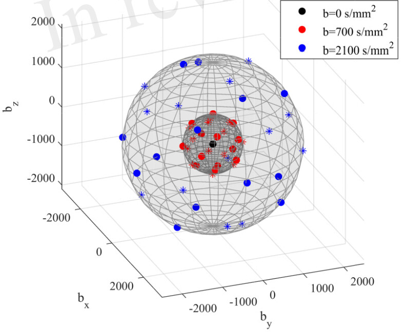
For the DW signal, we can safely assume antipodal symmetry, and hence any measurement along a given direction û is considered equivalent to a measurement in the opposite direction -û. In your plot, the blue dots are the actual directions recorded, the stars are their opposite counterparts; displaying both gives you a better idea of the actual coverage of the DW signal.
The way these schemes are typically optimised is via a bipolar electrostatic repulsion model: if we imagine each DW direction is represented by a stick through the origin with electric charges at either end, the aim is to find a configuration that places all these charges as far apart from each other as possible. Once we’ve done that, we can chose which end of each stick to use as our final direction – it doesn’t matter which as far as the DW signal is concerned, as the DW signal is symmetric and both orientations are equivalent. Note that this means we can pick all of the directions from the top hemisphere if we want to – and indeed you’ll find plenty of direction sets in common use that have done precisely this. But as far the sampling of the DW signal is concerned, this makes no difference (in theory).
Where the choice of polarity does matter however, is in the manifestation of artefacts such as eddy-current distortions: the opposite direction implies the opposite gradients, and this will lead to the opposite eddy-currents being induced, and hence the opposite distortions. When correcting for these distortions, this could mean that we end up with data with residual distortion relative to some undistorted external reference, because on average, the distortions in the DW data all tended to go one way. The FSL EDDY page has a good illustration of this. To avoid these kinds of biases, the recommendation is to make sure the directions do cover the full sphere relatively uniformly.
The way the gen_scheme script handles this is to first obtain an optimal distribution for DW signal sampling using a bipolar electrostatic model, and then pick polarities for these directions that maximise spherical coverage (via an unipolar electrostatic repulsion model). Because we’re using the original directions from the first stage and only changing their polarity, the uniformity of the DW sampling is unaffected by the second stage – but biases due to non-spherical coverage of the sampling are vastly minimised. Note that there’s no guarantee that they would be eliminated entirely, since that would entail changing the directions themselves, not just their polarity – and that would compromise the uniformity of the sampling of the DW signal, which in my opinion is by far the most important aspect. Others may have different opinions as to how best to balance these two considerations.
So to come back to your original question: the schemes produced by gen_scheme should cover the full sphere uniformly, in an optimal sense when assessed using a bipolar electrostatic model, and in an approximately optimal sense when assessed using a monopolar electrostratic model.
This can all be assessed using the dirstat command. Here’s an example output from the dHCP, and I’ll try to explain what everything means below:
dwi.mif (b=0) [ 20 volumes ]

dwi.mif (b=399.999982053125) [ 64 directions ]

  Bipolar electrostatic repulsion model:
    nearest-neighbour angles: mean = 18.0044, range [ 16.9147 - 18.8867 ]
    energy: total = 3680.82, mean = 115.026, range [ 114.685 - 115.455 ]

  Unipolar electrostatic repulsion model:
    nearest-neighbour angles: mean = 18.2928, range [ 16.9147 - 19.8795 ]
    energy: total = 1810.78, mean = 56.5868, range [ 54.0071 - 58.744 ]

  Spherical Harmonic fit:
    condition numbers for lmax = 2 -> 8: [ 1.00839 1.02292 1.05647 1.12811 ]

  Asymmetry of sampling:
    norm of mean direction vector = 0.0174578

dwi.mif (b=999.99994446477274) [ 88 directions ]

  Bipolar electrostatic repulsion model:
    nearest-neighbour angles: mean = 15.5307, range [ 14.8106 - 16.3173 ]
    energy: total = 7077.96, mean = 160.863, range [ 160.546 - 161.282 ]

  Unipolar electrostatic repulsion model:
    nearest-neighbour angles: mean = 15.6851, range [ 14.8106 - 17.2174 ]
    energy: total = 3482.04, mean = 79.1373, range [ 76.1162 - 81.9429 ]

  Spherical Harmonic fit:
    condition numbers for lmax = 2 -> 10: [ 1.00329 1.01312 1.02864 1.06596 1.17703 ]

  Asymmetry of sampling:
    norm of mean direction vector = 0.0155368

dwi.mif (b=2599.9999810546869) [ 128 directions ]

  Bipolar electrostatic repulsion model:
    nearest-neighbour angles: mean = 12.9365, range [ 12.3171 - 13.5842 ]
    energy: total = 15222, mean = 237.844, range [ 237.252 - 238.297 ]

  Unipolar electrostatic repulsion model:
    nearest-neighbour angles: mean = 13.208, range [ 12.3288 - 17.0051 ]
    energy: total = 7493.83, mean = 117.091, range [ 112.732 - 120.707 ]

  Spherical Harmonic fit:
    condition numbers for lmax = 2 -> 14: [ 1.00191 1.00791 1.02324 1.04504 1.08395 1.22253 2.15647 ]

  Asymmetry of sampling:
    norm of mean direction vector = 0.0152695
Here we have 4 sections, one for each shell in the DW scheme, sorted by b-value, and showing the number of DW directions in that shell. If you look at the last shell (b=2600s/mm²) for example, you’ll find:
-
Bipolar electrostatic repulsion model: an assessment of the coverage of the DW signal (i.e. assuming antipodal symmetry)
-
nearest-neighbour angles: the angle in degrees between each direction and its nearest neighbour on the sphere (or its opposite, since we assume antipodal symmetry). In your plots, that means the angles between any nearest pair of points, whether dots or stars. For a given number of directions, higher is generally better, and you want the [min max] range to be relatively tight around the mean (if the mininum is much smaller than the mean, that’s not a good sign).
-
energy: this is literally the cost function used in the optimisation of the directions. For a given number of directions, lower is better. You also get the average contribution per direction, along with the [min max] range. But it’s difficult to interpret these numbers unless you’re looking at straight comparisons between schemes.
-
Unipolar electrostatic repulsion model: an assessment of the coverage of the artefacts (i.e. not assuming antipodal symmetry)
-
nearest-neighbour angles: as for the previous sub-section, but this time ignoring the opposite directions. In your plot, that means the angles between any nearest pair of dots only, ignoring the stars. Again, for a given number of directions, higher is generally better, and you want the [min max] range to be relatively tight around the mean.
-
energy: as for the previous sub-section, but this time assuming a unipolar electrostatic repulsion model.
-
Spherical Harmonic fit:
-
condition numbers: this is probably the most relevant metric to look at when assessing the optimality of the sampling of the DW signal. It looks at the stability of the spherical harmonic fit up to the maximum harmonic order supported by the number of directions in that shell. Ideally, these conditions numbers should be close to 1 – higher numbers means noise in the signals translates to higher noise in the estimated coefficients. A poorly conditioned DW scheme might end up with very high condition numbers for the higher harmonic orders (I’ve seen some considerably higher than 10).
-
Asymmetry of sampling:
-
norm of mean direction vector: this is obtained by literally summing up all the direction vectors, and computing the amplitude of that sum (and normalising by the number of directions). It reflects the uniformity of the sampling over the full sphere. Larger values suggest an increasing susceptibility to artefacts such as residual distortions due to eddy-currents.
If the sampling covered the sphere uniformly, there would be equal contributions to that value from all directions – for every direction along +û, there would be a more or less equivalent direction pointing along -û – so on average, it should be close to zero.
A perfectly hemispheric scheme (e.g. optimised for uniformity of the DW sampling via a bipolar model, but picking all directions from one hemisphere) will generally have values close to 0.5. Values larger than that suggest a very messed up scheme…
OK, that’s probably already too much information, but hopefully your original question will have been answered somewhere in there…
Cheers,
Donald