Hi @stellamarissanchez89,
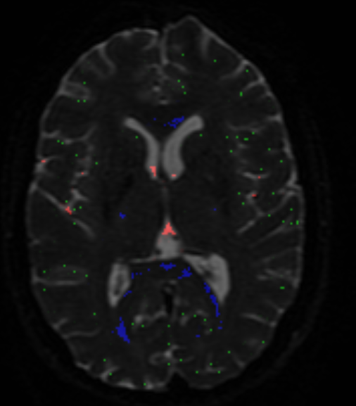
No worries at all: this is exactly how it should behave!  Essentially, the method is after the “purest” examples of voxels for each of the 3 tissue types (so it’s quite “picky” on purpose), but at the same time it of course also wants a decent number of voxels for each, so the response functions can be estimated robustly in terms of shape (angular and b-value contrast) as well as size/scale. But to actually put you a bit more at ease: you may get the wrong idea about the numbers of voxels you’re looking at in that image! This looks like an HCP dataset, am I right? Or at least one with a similarly high spatial resolution (i.e. ~ 1.25mm isotropic?). See here a result I got for an HCP dataset:
While these results may at first glance look quite sparse (and they are, compared to the whole volume), the numbers of voxels selected for each tissue type may surprise you. In this case they were:
- (single fibre) WM (blue): 1570 voxels
- GM (green): 2794 voxels
- CSF (red): 1824 voxels
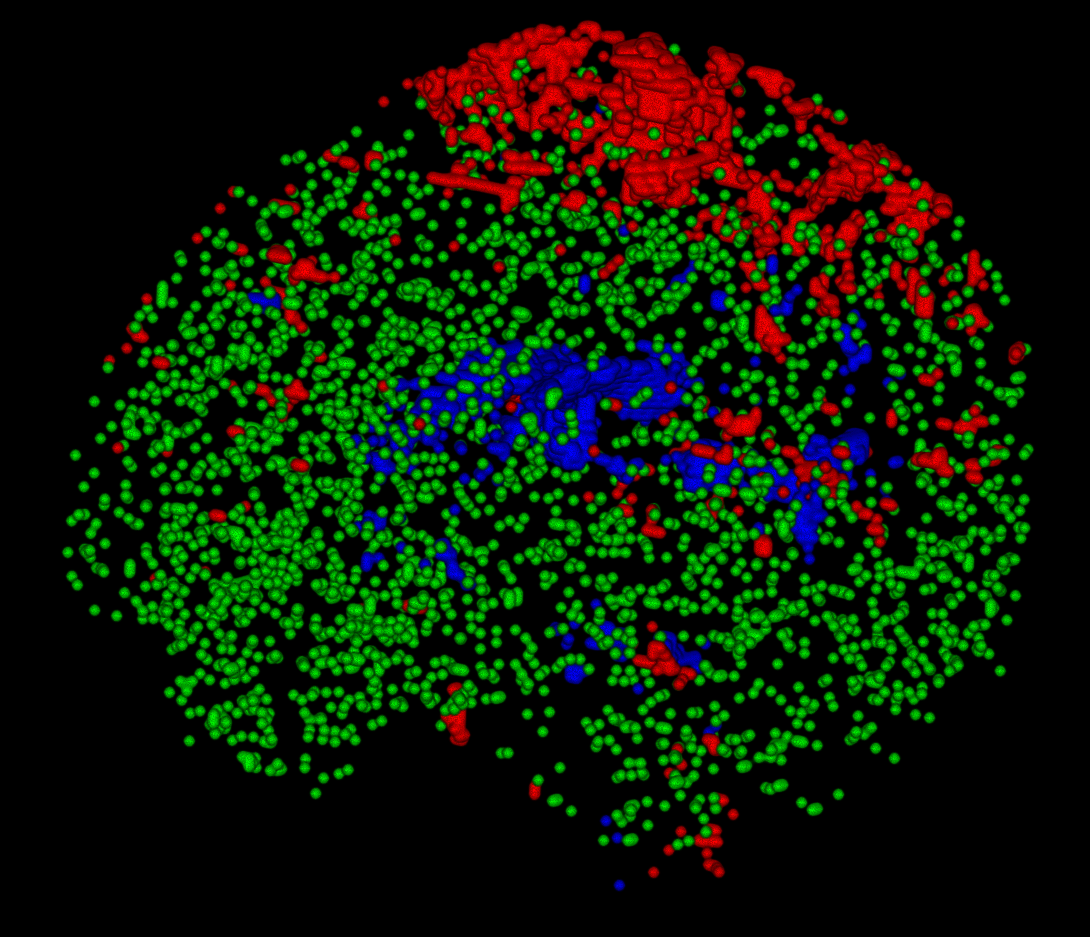
To get a better impression of how these are really distributed over the whole volume, rather than just looking at a single slice, you can open up the voxels image directly in the viewer (i.e. not as an overlay to a b=0 image), and switch to the volume render view (and changing the intensity range a bit to crank up the brightness/contrast; I’ve set the range to 0 - 0.5 below):
You’ll see for instance that (at this spatial resolution, but most things hold for other resolutions as well):
- The single fibre WM is typically sourced in similar structures in healthy subjects. A prominent part will be bits of the corpus callosum (especially the splenium at times), but strikingly the actual “exact” mid-sagittal bit is quite often not included (due to, apparently but not entirely surprisingly, slightly higher dispersion compared to the bits of the CC just to the sides of the mid-sagittal plane).
- Due to where GM naturally appears (the cortex, that is relatively thin and has at typical resolutions a lot of partial volume with either the on the inside or CSF on the outside), the GM voxels are typically a nice big cloud of green dots, most of which are not connected to each other in clusters.
- The CSF is not per se mostly sourced from the ventricles, especially in younger subjects where the ventricles are actually quite small an a lot of partial voluming is going on with the WM on all edges. Also, as HCP data nicely shows you, you’ve got the choroid plexus filling up quite some space in those posterior bits of the ventricles; so again, these voxels aren’t always the best ones to source the CSF response.
The command line output of dwi2response dhollander also shows you how many voxels got selected for each tissue type (as well as how many voxels were still present along certain steps throughout the algorithm). Look for something like this close to the end of the command line output:
dwi2response: Summary of voxel counts:
dwi2response: Mask: 95148 --> 69172 --> 69172
dwi2response: WM: 39444 --> 36473 --> 182 (SF)
dwi2response: GM: 24516 --> 15982 --> 320
dwi2response: CSF: 5212 --> 1883 --> 188
This particular example was from a run on more “conventional” data with a spatial resolution of 2.5 mm isotropic; the subject was a healthy young adult person. The final numbers of voxels selected for (single fibre) WM, GM and CSF were 182, 320 and 188. These numbers are on the order of magnitude of about a bit more than 8 times less than the above HCP dataset (since, at this spatial resolution, there’s about 8 times less voxels in a typical brain mask). The numbers may also vary among the tissue types as well, depending on the “availability” of each tissue type in a given subject. A subject with a lot of WM atrophy may give you relatively less single fibre WM voxels, but in case of a lot of overall brain atrophy (and e.g. severely enlarged ventricles), you may get more CSF voxels, etc…
For yet another example, see the images on the right side in the original abstract of the method.
But it’s still a very good idea to actually check that voxels image (as you did); it’s there as an output on purpose, particularly with quality assessment in mind!
Cheers,
Thijs
 Essentially, the method is after the “purest” examples of voxels for each of the 3 tissue types (so it’s quite “picky” on purpose), but at the same time it of course also wants a decent number of voxels for each, so the response functions can be estimated robustly in terms of shape (angular and b-value contrast) as well as size/scale. But to actually put you a bit more at ease: you may get the wrong idea about the numbers of voxels you’re looking at in that image! This looks like an HCP dataset, am I right? Or at least one with a similarly high spatial resolution (i.e. ~ 1.25mm isotropic?). See here a result I got for an HCP dataset:
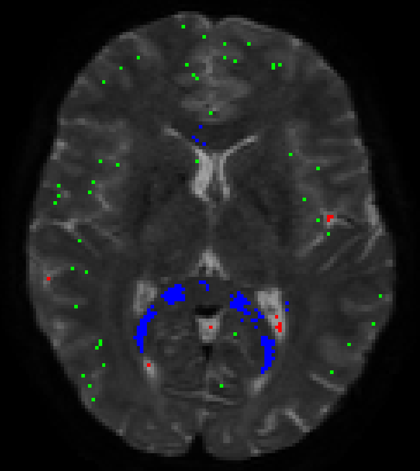
 , but now is clearer
  .
.