Thanks for your reply!
I’m not exactly sure where the bvecs for 7T came from, I’ll have to double check.
Apparently there is some sort of scaling/alteration going on for the bvecs on 7T cause these are the bvecs that were put into the scanner:
0.00000, 0.00000, 0.00000, 0.00000
0.00000, 0.00000, 0.00000, 0.00000
0.00000, 0.00000, 0.00000, 0.00000
0.00000, 0.00000, 0.00000, 0.00000
0.14600, -0.04100, -0.98900, 2500
-0.19300, 0.97900, -0.06900, 2500
-0.90800, -0.39200, -0.14500, 2500
-0.84300, 0.42600, 0.33100, 2500
-0.57800, 0.34500, -0.74000, 2500
0.49700, 0.68500, -0.53200, 2500
0.23500, 0.72100, 0.65200, 2500
-0.79300, -0.11700, 0.59800, 2500
-0.72500, 0.63800, -0.25900, 2500
-0.60100, -0.27600, -0.75000, 2500
0.37200, -0.70700, -0.60200, 2500
0.04600, -0.75100, 0.65800, 2500
-0.51000, -0.85700, -0.08000, 2500
0.97300, -0.11700, 0.19800, 2500
-0.26700, -0.36500, 0.89200, 2500
0.50800, -0.31400, -0.80200, 2500
0.05200, 0.95600, 0.28800, 2500
-0.30600, 0.03800, -0.95100, 2500
 0.85700, 0.44200, -0.26700, 2500
-0.57300, 0.80700, 0.14100, 2500
-0.65800, -0.59300, -0.46400, 2500
0.41000, -0.74600, 0.52500, 2500
-0.01900, -0.44300, -0.89600, 2500
0.23400, 0.92700, -0.29200, 2500
0.97800, -0.04000, -0.20500, 2500
-0.82500, 0.05400, -0.56400, 2500
-0.14100, 0.42400, -0.89400, 2500
-0.54300, -0.10000, 0.83400, 2500
0.27900, -0.89500, -0.34600, 2500
0.67400, 0.72000, -0.16500, 2500
-0.89500, 0.44500, -0.03500, 2500
-0.33200, -0.38800, -0.86000, 2500
0.75800, -0.26300, -0.59700, 2500
0.11900, -0.91900, 0.37600, 2500
-0.85800, -0.26700, -0.43900, 2500
0.60300, 0.43600, -0.66800, 2500
-0.36400, -0.85300, -0.37600, 2500
-0.78000, 0.41000, -0.47100, 2500
-0.25300, 0.52300, 0.81400, 2500
0.22100, 0.64300, -0.73300, 2500
0.49200, -0.85400, 0.17000, 2500
0.97600, 0.20400, -0.07600, 2500
-0.63500, 0.63400, 0.44100, 2500
-0.57600, 0.05400, -0.81600, 2500
-0.19800, -0.98000, -0.00900, 2500
-0.02600, 0.16800, -0.98600, 2500
0.73400, 0.65700, 0.17100, 2500
0.04900, -0.77500, -0.63000, 2500
0.36600, -0.56000, 0.74300, 2500
0.89500, -0.07400, -0.44000, 2500
-0.36200, 0.13800, 0.92200, 2500
0.48400, 0.56800, 0.66600, 2500
0.46800, 0.82700, -0.31200, 2500
0.76600, -0.63500, -0.09600, 2500
0.95800, 0.10200, 0.26900, 2500
0.12400, 0.18400, 0.97500, 2500
0.78000, 0.38900, -0.49000, 2500
-0.61100, 0.59600, -0.52100, 2500
0.31200, -0.94300, -0.12100, 2500
0.16900, 0.82900, -0.53400, 2500
0.00000, 0.00000, 0.00000, 0.00000
0.00000, 0.00000, 0.00000, 0.00000
0.97200, 0.19000, 0.13600, 1000
0.02500, -0.66500, 0.74700, 1000
0.22000, -0.72500, -0.65300, 1000
-0.68200, -0.06600, 0.72900, 1000
0.36300, 0.92800, 0.08100, 1000
-0.53800, 0.00900, -0.84300, 1000
0.70600, -0.70600, 0.05100, 1000
-0.05300, 0.18700, 0.98100, 1000
0.69900, 0.62400, -0.34900, 1000
-0.23300, 0.94500, -0.23000, 1000
0.55800, 0.56900, 0.60400, 1000
0.91600, -0.28400, -0.28500, 1000
0.72200, -0.42000, 0.55000, 1000
0.36700, 0.41400, -0.83300, 1000
0.13100, -0.95100, -0.28100, 1000
-0.60100, 0.44400, 0.66400, 1000
-0.77700, -0.60600, -0.17100, 1000
0.20100, -0.28100, 0.93800, 1000
0.94200, -0.24600, 0.22800, 1000
0.26800, 0.87000, -0.41400, 1000
0.18900, 0.55200, 0.81200, 1000
0.91200, 0.20300, -0.35700, 1000
-0.43500, 0.69100, -0.57800, 1000
-0.56600, 0.75600, 0.32800, 1000
-0.79900, -0.18600, -0.57200, 1000
0.35700, -0.00600, -0.93400, 1000
-0.24800, -0.85500, -0.45500, 1000
0.48600, 0.62200, -0.61400, 1000
-0.31900, -0.22800, -0.92000, 1000
0.05400, 0.99500, -0.09000, 1000
and these are the bvces in the dicomheader:
0 0 0 0
0 0 0 0
0 0 0 0
0 0 0 0
-0.23607109 -0.52415819 0.81824729 2510
0.89302078 0.25900593 0.36800791 2495
0.79618374 -0.12902996 0.59113681 2495
0.23396394 0.9298547700000001 -0.28395593 2495
0.93568576 0.13995296 0.32389092 2505
-0.50582701 0.84471002 0.17494001 2500
-0.34621991 0.84753877 -0.40225589 2490
0.45696822 -0.6309563 -0.6269563 2490
0.48699677 0.38899682 0.78199464 2495
0.61784501 -0.67283101 0.406898 2505
-0.57698421 -0.10499704 0.8099783 2505
-0.82669461 -0.52080775 -0.2129209 2490
0.89371183 -0.03998699 0.44685591 2500
-0.29010089 -0.5411888 -0.78927571 2495
0.11595099 -0.96259094 -0.24489599 2485
-0.80018196 -0.40309198 0.44410098 2505
-0.513981 0.83997001 -0.173994 2490
0.78854813 0.15291203 0.5956591 2505
-0.9492796 0.2330689 0.21106191 2500
0.23296404 0.78288015 -0.5769111099999999 2490
0.02099901 -0.18799008 0.98194642 2500
-0.21693198 -0.95570089 -0.19893798 2490
0.77400322 -0.60400217 0.19000105 2505
-0.16092797 0.35583994 0.92058684 2495
-0.14703502 -0.7311731 0.66615809 2500
0.8881412400000001 0.41706611 0.19303105 2505
0.5619707900000001 0.23198792 0.79395871 2500
0.3808088 -0.14292792 -0.91354051 2490
-0.30600002 -0.19900001 0.93100106 2500
-0.33208601 0.130034 0.93424303 2495
0.96322645 0.26506212 0.04401002 2495
0.95950146 -0.2051071 0.19310109 2505
-0.45296484 -0.88893168 0.06799498 2505
-0.77313264 -0.62810771 -0.08801496 2495
0.70908181 -0.40804689 0.5750658400000001 2500
-0.69276918 0.02399201 0.72076019 2500
0.6816591 -0.52873507 0.50574707 2505
0.14199506 0.72497632 0.67397829 2495
0.74016829 0.38808815 -0.54912521 2485
-0.10300599 0.82204393 0.56002995 2500
-0.58403697 -0.59603797 -0.55103498 2495
-0.08800798999999999 0.33503095 0.93808787 2495
0.55226287 0.79237682 -0.25912294 2490
0.83815768 0.45808582 0.29605589 2505
0.36299507 -0.5609931 0.74399014 2495
0.18406204 0.39213308 0.90130617 2510
-0.72093807 0.69294107 -0.008999 2490
-0.43310105 -0.68215907 0.58913706 2505
-0.50211396 -0.6901569400000001 -0.52111896 2490
-0.17094403 -0.50883308 0.84372213 2500
0.46296784 0.42297085 -0.77894572 2485
-0.38503005 0.80906411 -0.44403506 2490
-0.71310197 0.24703499 0.65609397 2500
-0.25992306 -0.8847372100000001 0.38688509 2495
-0.001 0.07700203 -0.99703043 2495
-0.03700201 0.90205736 -0.43002717 2485
-0.57032021 0.30317011 0.76342828 2500
0.28210511 0.14505406 0.9483543800000001 2500
-0.7210980299999999 -0.60808202 0.33204501 2500
-0.26698506 0.95994522 0.08499502 2505
0 0 0 0
0 0 0 0
-0.5773502700000001 0.5773502700000001 -0.5773502700000001 995
-0.5773502700000001 -0.5773502700000001 -0.5773502700000001 995
-0.5773502700000001 -0.5773502700000001 0.5773502700000001 1005
0.5773502700000001 -0.5773502700000001 -0.5773502700000001 995
-0.5773502700000001 0.5773502700000001 -0.5773502700000001 995
0.5773502700000001 -0.5773502700000001 0.5773502700000001 1005
-0.5773502700000001 -0.5773502700000001 -0.5773502700000001 1000
0.5773502700000001 0.5773502700000001 -0.5773502700000001 990
-0.5773502700000001 0.5773502700000001 0.5773502700000001 1000
0.5773502700000001 0.5773502700000001 0.5773502700000001 1000
-0.5773502700000001 0.5773502700000001 -0.5773502700000001 995
-0.5773502700000001 -0.5773502700000001 0.5773502700000001 1000
-0.5773502700000001 -0.5773502700000001 -0.5773502700000001 995
-0.5773502700000001 0.5773502700000001 0.5773502700000001 1005
-0.5773502700000001 -0.5773502700000001 0.5773502700000001 1000
0.5773502700000001 0.5773502700000001 -0.5773502700000001 995
0.5773502700000001 -0.5773502700000001 0.5773502700000001 1000
-0.5773502700000001 -0.5773502700000001 -0.5773502700000001 990
-0.5773502700000001 -0.5773502700000001 -0.5773502700000001 1000
-0.5773502700000001 0.5773502700000001 0.5773502700000001 1000
-0.5773502700000001 0.5773502700000001 -0.5773502700000001 995
-0.5773502700000001 0.5773502700000001 0.5773502700000001 1000
0.5773502700000001 0.5773502700000001 0.5773502700000001 1005
0.5773502700000001 0.5773502700000001 -0.5773502700000001 995
0.5773502700000001 -0.5773502700000001 0.5773502700000001 1005
-0.5773502700000001 -0.5773502700000001 0.5773502700000001 1005
0.5773502700000001 -0.5773502700000001 0.5773502700000001 1005
-0.5773502700000001 0.5773502700000001 0.5773502700000001 1005
0.5773502700000001 -0.5773502700000001 0.5773502700000001 1005
-0.5773502700000001 0.5773502700000001 0.5773502700000001 1000
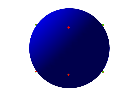
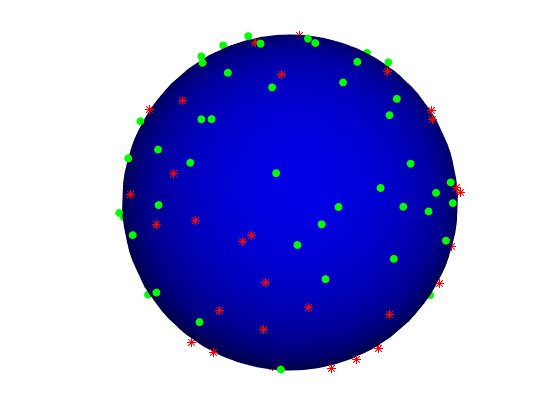
The distribution for the b1000 shell in the header is especially strange to me. This is what the dirstat output looks like for the bvecs that were originally fed into the scanner:
b = 0 [ 2 directions ]

  Bipolar electrostatic repulsion model:
    nearest-neighbour angles: mean = 180, range [ 180 - 180 ]
    energy: total = inf, mean = inf, range [ 1.79769e+308 - inf ]

  Unipolar electrostatic repulsion model:
    nearest-neighbour angles: mean = 180, range [ 180 - 180 ]
    energy: total = inf, mean = inf, range [ 1.79769e+308 - inf ]

  Spherical Harmonic fit:
    condition numbers for lmax = 2 -> 0:


b = 1000 [ 30 directions ]

  Bipolar electrostatic repulsion model:
    nearest-neighbour angles: mean = 22.8068, range [ 18.5946 - 28.4905 ]
    energy: total = 768.879, mean = 51.2586, range [ 49.4739 - 53.0132 ]

  Unipolar electrostatic repulsion model:
    nearest-neighbour angles: mean = 24.5593, range [ 18.5946 - 33.7788 ]
    energy: total = 382.302, mean = 25.4868, range [ 21.5679 - 30.1538 ]

  Spherical Harmonic fit:
    condition numbers for lmax = 2 -> 6: 1.12489 1.32071 4.17052

b = 0 [ 4 directions ]

  Bipolar electrostatic repulsion model:
    nearest-neighbour angles: mean = 180, range [ 180 - 180 ]
    energy: total = inf, mean = inf, range [ 1.79769e+308 - inf ]

  Unipolar electrostatic repulsion model:
    nearest-neighbour angles: mean = 180, range [ 180 - 180 ]
    energy: total = inf, mean = inf, range [ 1.79769e+308 - inf ]

  Spherical Harmonic fit:
    condition numbers for lmax = 2 -> 0:


b = 2500 [ 60 directions ]

  Bipolar electrostatic repulsion model:
    nearest-neighbour angles: mean = 15.9921, range [ 13.0323 - 19.9187 ]
    energy: total = 3233.96, mean = 107.799, range [ 106.246 - 110.073 ]

  Unipolar electrostatic repulsion model:
    nearest-neighbour angles: mean = 17.8404, range [ 13.2477 - 28.425 ]
    energy: total = 1623.74, mean = 54.1246, range [ 45.6541 - 61.2573 ]

  Spherical Harmonic fit:
    condition numbers for lmax = 2 -> 8: 1.04723 1.17954 1.32747 2.5837
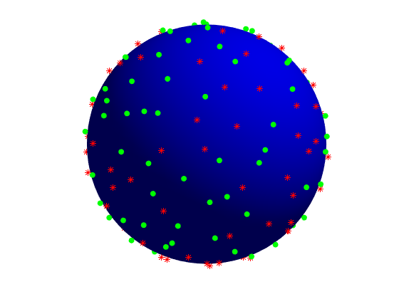
These ones still don’t look too pretty but it at least looks better than the bvecs coming out of the scanner and into the dicom header. Any clue about why, especially the b1000 shell, looks so strange? I know it’s better not the change the bvecs manually and use the ones directly from the image header but would it in this case be a good idea to use the original bvecs instead of the header ones?
Cheers!
 ) my 7T set came out like this: