Thanks zeydabadi,
As you mentioned, 5tt_noncoreg.nii.gz is a 4D volume. As 5tt_noncoreg.nii.gz is derived from T1_raw.mif (a 3D image), here should I have used T1_raw.mif (or nii.gz) instead of 5tt_noncoreg.nii.gz?
I have confirmed mean_b0_preprocessed.nii.gz is a 3D volume.
I assume you should you use the 5tt_noncoreg.nii.gz but why it’s not in 3D, I don’t know. Maybe the Marlene can help.
Thanks Mahmoud,
I think 5tt_noncoreg.nii.gz provided in Supplementary_Files have 5 volumes(, which means this is a 4D image), too. So I wonder I shouldn’t use 5tt_noncoreg.nii.gz here. Am I right? I would appreciate it if I could receive a comment from Marlene.
Hi Mahmoud,
You can use labelconvert to do this. I show how to use this for the HCPMMP1 atlas in the tutorial. The procedure for the AAL atlas is very similar to this (section 8.1 in the appendix). However, a few things are different for the AAL atlas:
The AAL is – unlike the surface-based HCPMMP1 atlas – a volumetric atlas. This makes things easier for you since you do not have to do the FreeSurfer anatomical preprocessing in this case. However, you still have to register the AAL to the highresolution native T1 space in a first step (the AAL atlas is in standard space: MNI_152_2mm). There are several ways to do this, e.g. with MRtrix or FSL commands. I like to use FSL’s flirt tool for this. Here are a couple of commands with which you can achieve this (assuming you have done FSL’s anatomical preprocessing, which gave you a T1_biascorr_brain.nii.gz, and the AAL file in standard space is called “AAL.nii”):
flirt –in T1_biascorr_brain.nii.gz –ref $FSL_DIR/standard/MNI152_2mm_brain.nii.gz –omat highres2standard.mat –interp nearestneighbour –datatype int -inverse
convert_xfm –omat standard2highres.mat –inverse highres2standard.mat
flirt –in AAL.nii –ref T1_biascorr_brain.nii.gz –out aal2highres.nii.gz –applyxfm –init standard2highres.mat –interp nearestneighbour
You can then use labelconvert with the resultant file, e.g.
labelconvert aal2highres.nii.gz aalLUT_90_orig.txt aalLUT_90_ordered.txt aal2highres.mif
(In case you do not have these files, I uploaded the following three files on the OSF website: aalLUT_90_orig.txt, aalLUT_90_orig.txt, and AAL.nii. You can find those in the Supplementary Files directory here: OSF. However, please note that the color lookup tables I provide are for the 90 parcellation AAL atlas, and I ask you to verify it before using it).
Regarding your second question,
I think using the AAL to identify the CST is not the way to go. I’m not an expert here, but aren’t there any atlases of white matter pathways? Alternatively, you could try to identify the CST in every of your subjects by tracking through a ROI (in the white matter) through which you know the CST must pass (e.g. how in section 4.4 in the tutorial, which shows how to use tckedit to identify the CST). However, this is a subjective procedure, so I recommend this only as an exploratory analysis. An atlas would be the preferrable option for a standardized analysis.
Hope this helps.
Cheers,
Marlene.
2 Likes
Hi @tkimura,
the problem here is indeed the latest version of FSL (which I guess you have) expects a single 3D volume as a fieldmap (the old version would only read the first volume if the fieldmap was 4D; for another discussion on this see https://www.jiscmail.ac.uk/cgi-bin/webadmin?A2=FSL;1e8be9c7.1811). One easy way around this is to split the 4D 5tt_nocoreg.nii.gz into 3D volumes. This can be achieved, e.g. with fslsplit:
fslsplit 5tt_nocoreg.nii.gz myprefix -t
This command will split the 5tt_nocoreg-image into 5 3D volumes, where “prefix” denotes the prefix of each of the volumes (like this, your outputs will be called “prefix0000.nii.gz” for the first 3D volume of 5tt_nocoreg, “prefix0001.nii.gz” for the second volume, etc.). Now you can use either of those 3D images with flirt, e.g.
flirt -in mean_b0_preprocessed.nii.gz -ref prefix0000.nii.gz -interp nearestneighbour -dof 6 -omat diff2struct_fsl.mat
I now this is a little complicated, but the best way I can think of right now. Let me know if you find a quicker way. However, I just ran these commands myself and can confirm that they work and that the resulting diff2struct_fsl.mat is correct.
Hope this helps.
Cheers,
Marlene.
5 Likes
Hi Marlene,
Thanks for your helpful comment. Now command flirt works without error. But I checked the results and found that 5tt_noncoreg.mif has wrong direction (axial image has changed to saggital). As maybe I did something wrong, I will try to fix and let you know.
Takashi
1 Like
You definitely don’t want to be using the 5 separate tissue partial volume images for registration: apart from the fact that the registration algorithm may not be able to find a good alignment between an individual tissue image and a template T1-weighted image based on its internal image matching cost function, resulting in a bad alignment, doing this five separate times would give you five tissue images with five different transforms!
You want to perform the registration using the most appropriate images for such (e.g. T1-weighted image & mean b=0 image), and then apply the transformation that was optimised by the registration algorithm to any other images that you wish to undergo the same transformation. I.e. If your 5TT image is intrinsically aligned with the T1 image data (given it was calculated from such), and you then estimate a transformation that aligns the T1 image with the DWI data, then applying that same transformation to the 5TT image will make those data also align with the DWIs.
1 Like
Hi Marlene,
Excellent tutorial, I didn’t realize MRTrix had so many capabilities!
A few quick questions:
-
Does MRTrix have any graphical interface for drawing ROIs manually?
-
When tracking, you showed the use of anatomical constraints to ensure streamlines start and end at the WM/GM interface. Then used cortical (or sub-cortical) labels for connectome generation. What happens if the streamlines stop just short of labels (for example if my labels don’t exactly align or match the WM/GM boundary)? Will they not be counted in the connectome generation?
-
Does MRTrix have any capabilities for connectome generations using meshes as opposed to labels? For example mesh of WM/GM interface or mid-cortex mesh. Similarly, can meshes be used, for use with anatomical constrained tractography, or should this be converted to binary masks?
Thank you very much,
Kurt
Does MRTrix have any graphical interface for drawing ROIs manually?
In mrview, click the “Tools” button on the toolbar, then select “ROI tool”. You can open existing ROIs or create new ones, and activate editing by clicking the “Edit” button within that tool.
What happens if the streamlines stop just short of labels (for example if my labels don’t exactly align or match the WM/GM boundary)? Will they not be counted in the connectome generation?
tck2connectome by default will search for any labelled voxel within a 2mm radius of the streamline termination point, precisely for this reason.
Does MRTrix have any capabilities for connectome generations using meshes as opposed to labels?
Not yet. But if the parcels are relatively large, then the difference in outcome between using a native mesh representation and using a voxel-based representation of such should be minimal.
Similarly, can meshes be used, for use with anatomical constrained tractography, or should this be converted to binary masks?
Again, not yet. But ACT does not require the tissues to be defined as binary masks: a partial volume fraction representation means that complex shapes of tissue interface surfaces can be represented without too much loss of precision.
Hi @schilkg1,
While it might be inappropriate to have a lengthy discussion within this post, I do wish to clarify some points respecting your 2nd and 3rd questions. Please see below.
Good question. We did have spotted on the misalignment issue that you mentioned here; indeed, only ~25% of streamlines will be used in the connectome largely because of such misalignment. We describe it as a source data mismatch problem: the WM/GM boundary derived from tissue partial volume maps (based on tissue segmentation) used in tractography is not always consistent with the boundary of brain parcellation images used in connectome construction. Performing a 2-mm search from streamline endpoints (to find the nearest labelled voxel ) is the current MRtrix3’s default mechanism implemented in tck2connectome to deal with such inconsistencies (see the -assignment_radial_search in the help page of tck2connectome). Using the radial search, ~85% of streamlines will contribute to the outcome connectome. If interested, please see this abstract for the relevant influences.
To avoid losing precision, my approach to deal with the source data mismatch is directly using high-resolution tissue surface meshes to unify the source data: the same labelled surfaces are used for both tractography and connectome generation, as described in your question. I called this method Mesh-based ACT (or MACT), where streamline endpoints are the intersection points between streamlines and the labelled surfaces (cortical and sub-cortical WM/GM surfaces). When using MACT for connectome generation, there is no need to convert, for example, the vertex-wise labels of HCP-MMP into volume-based labelled images.
For more details, please see MACT abstract for reference. If you registered the ISMRM2017 meeting, I think my presentation video (0058) should still be accessible, there are more explanations on the background and the principle of MACT.
Finally, about using a mid-cortex mesh, I believe that it would only require a simple change in MACT. Coincidentally, I did once consider using a mid-cortex mesh as a default setting (rather than taking both inner and outer cortical GM surfaces). If you or anyone see any potential benefits or applications of using mid-cortex, I’d love to hear your insights and recommendations. So, even though MACT is not yet available in MRtrix3, it has already and still received serious development by me and has been applied to a few studies. Any queries about MACT are very much welcome; please let me know via a personal message or an email.
Many thanks.
1 Like
Hi rsmith, I am having the same issue as tkimura I think.
I am hoping someone can help me to operationalise the following instructions you provided?
If your 5TT image is intrinsically aligned with the T1 image data (given it was calculated from such), and you then estimate a transformation that aligns the T1 image with the DWI data, then applying that same transformation to the 5TT image will make those data also align with the DWIs
Sorry but I’m a bit of a novice.
Thank you, Dan
okay, I have run the command again using the myprefix0000.nii.gz rather than the myprefix0001.nii.gz file and it worked. I’m not sure why this is the case though? If anyone has the time to reply that would be great. Kind regards, Daniel123
Hi Daniel,
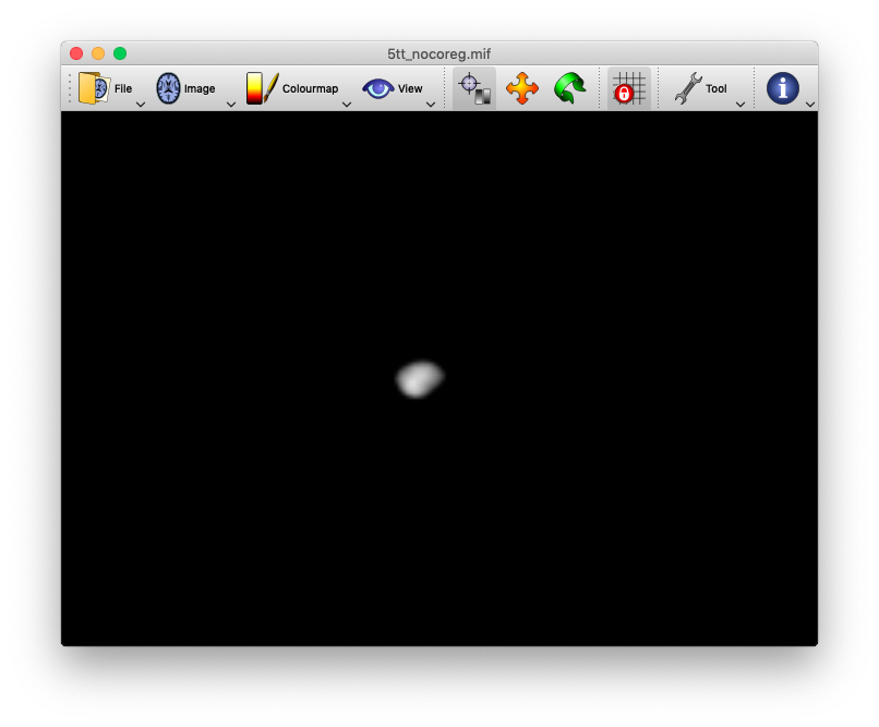
the reason why it works with the myprefix0000.nii.gz is that this is the 3D volume where the cortical gray matter boundaries are specified (see upper image). The myprefix0001.nii.gz defines the subcortical gray matter boundaries (see lower image). If we continue this, the myprefix0002.nii.gz, will specify the white matter regions, and so on). I guess by looking at the pictures it should be clear why using the myprefix0001 does not work for a proper registration.

However, as @rsmith suggested above, the better idea might be to use the T1 as a reference image all along.
2 Likes
I am hoping someone can help me to operationalise the following instructions you provided?
If your 5TT image is intrinsically aligned with the T1 image data (given it was calculated from such), and you then estimate a transformation that aligns the T1 image with the DWI data, then applying that same transformation to the 5TT image will make those data also align with the DWIs
This is me providing a precise description such that anyone who does the wrong thing is technically disobeying my instructions, while minimising length because time is finite; I do that a lot. I’ll try to contextualise why I put it this way:
Consider doing your processing steps in this order:
-
Generate a 5TT image from the T1.
-
Perform registration between DWI and T1 data to estimate the spatial transformation that gets them aligned.
-
Transform T1 data in space in order to get it aligned with the DWI data.
-
Perform ACT using DWI data and the 5TT image.
The issue is that the DWI data and the 5TT image still don’t align with one another; so ACT will appear to be doing completely the wrong thing.
Upon generating a 5TT segmentation image from a T1-weighted image, those two images intrinsically align with one another in space, since one was generated directly from the other.
The reason I worded the quoted text in that way is because in this scenario, step 3 needs to be applied to the 5TT image also, in order to transform that information in space to align with the DWI data. However, step 2 should not be performed separately for the 5TT image. There is a single unique spatial transformation that is required to achieve alignment between DWI (and derived) data and T1-weighted (and derived) data, and that transformation (as estimated through registration) should be done using the image information most appropriate for that task (that’s the T1-weighted image, not the 5TT image). Once that transformation is estimated, it can be applied to any image for which undergoing that transformation is deemed appropriate.
2 Likes
Hi experts,
When I follow the appendix of the tutorial to prepare parcellation image for structural connectivity analysis, I encountered one problem.
The tutorial said two annotation files of the HCP MMP 1.0 atlas named “lh/rh.hcpmmp1.annot” should be copied under path: $SUBJECTS_DIR/fsaverage/label/, but why at the 3rd step the command, the file is “$SUBJECTS_DIR/fsaverage/label/lh.glasser.annot”, I really don’t know how I can generate the “lh.glasser.annot” files.
Thanks.
Huan
Hi Huan!
Thanks for paying attention. The file name of the command should of course read “lh/rh.hcpmmp1.annot”. I’m referring to the exact same files, but accidentally was inconsistent with the naming. So you can just copy the rh/lh.hcpmmp1.annot files into the $SUBJECTS_DIR and the use the command with lh/rh.hcpmmp1.annot instead of lh/rh.glasser.annot.
Sorry for causing this confusion 
Marlene
1 Like
I have two questions:
- Is there any difference of the 5TT image: one is directly generated from the T1 (registrated to B0 firstly), and the other is generated from T1(not registrated to B0) and then registrated to B0 by the transformation matrix of T1 to B0? And If there is difference, which step is recommended?
- Should I bet T1 and b0 image before the registration?
Hi Marlene,
First, thank you very much for a great tutorial. I have processed connectivity analysis using HCP surface atlas and I want to generate Fornix tract (connectome2tck). Do you have any idea which nodes are connected through this tract? I have looked for the literature and it connects Hippocampus and other region but I don’t know what is the other region?
Thanks,
Cmid
Hi Cmid,
the fornix connects parts of the hippocampus to the mammillary bodies. The hippocampus is already included in the HCPMMP1-parcellation in the tutorial. However, the mammilary bodies are not. There is a very nice subcortical atlas provided by Ewert et al. (2017, Neuroimage), which provides very fine-grained parcellations of many subcortical structures, including the mammilary bodies. This atlas can be downloaded from here: https://www.lead-dbs.org/helpsupport/knowledge-base/atlasesresources/atlases/. Just identify the mammilary bodies there and register them to your diffusion image; then track between those two nodes.
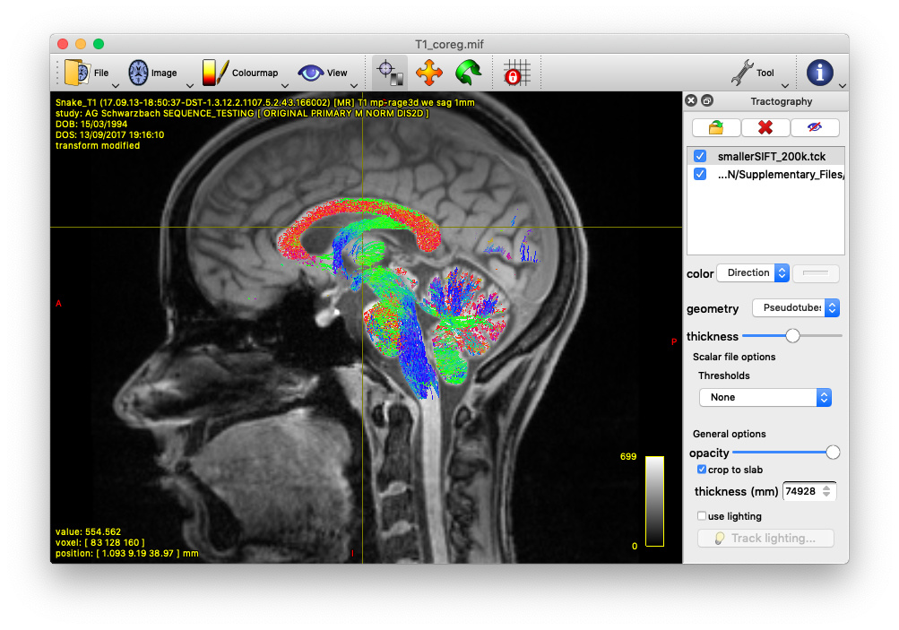
Alternatively, you could also track the fornix by using tckedit with a ROI through which you know the fornix passes. I’m providing an example below (based on the tutorial data). In the first image, I loaded the sift_1mio.tck onto the T1_coreg.mif. There I found that the fornix passes through the coordinates 0.31,11.76,37.32. Then I used tckedit as follows
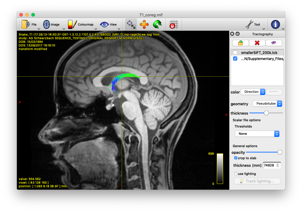
tckedit -include 0.31,11.76,37.32,3 sift_1mio.tck fornix.tck
to obtain the second image. Admittedly, this is just a quick & dirty approach to identify the fornix, but depending on your question, this might be enough. In any case, I would go for the Ewert atlas also.
Cheers,
Marlene
Hey @martahedl,
hey @rsmith,
thanks for the great tutorial.
To register to the T1 image instead of the 5tt I adapted the commands to:
flirt -in mean_b0_preprocessed.nii.gz -ref T1_raw.nii.gz -interp nearestneighbour -dof 6 -omat diff2struct_fsl.mat

transformconvert diff2struct_fsl.mat T1_raw.nii.gz mean_b0_preprocessed.nii.gz flirt_import diff2struct_mrtrix.txt

mrtransform 5tt_nocoreg.mif -linear diff2struct_mrtrix.txt -inverse 5tt_coreg.mif -flip 0
This is the original code from the tutorial:
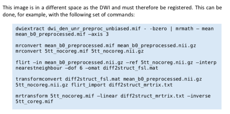
Is my adaption correct?
For some reason I had to include the flip argument to get the same orientation as the other images. Do you know why or if I made a mistake?
Thanks for your help!
Best Regards,
Darius